Clustering Algorithms
Introduction
Clustering is an unsupervised machine learning technique that groups similar data points together into clusters based on their characteristics, without using any labeled data. The objective is to ensure that data points within the same cluster are more similar to each other than to those in different clusters, enabling the discovery of natural groupings and hidden patterns in complex datasets.
Goal: Discover the natural grouping or structure in unlabeled data without predefined categories.
How: Data points are assigned to clusters based on similarity or distance measures.
Similarity Measures: Euclidean distance, cosine similarity, or other metrics depending on data type and clustering method.
Output: Each group is assigned a cluster ID representing shared characteristics within the cluster.
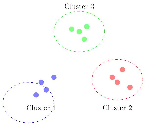
Example: Customer Purchase Data
If we have customer purchase data, clustering can group customers with similar shopping habits. These clusters can then be used for targeted marketing, personalized recommendations, or customer segmentation.
Types of Clustering
1. Hard Clustering
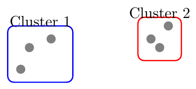
In hard clustering, each data point strictly belongs to exactly one cluster, no overlap is allowed. This approach assigns a clear membership.
Example: If clustering customer data into 2 segments, each customer belongs fully to either Cluster 1 or Cluster 2.
Use Cases: Market segmentation, customer grouping, document clustering.
Limitations: Cannot represent ambiguity or overlap; boundaries are crisp.
2. Soft Clustering
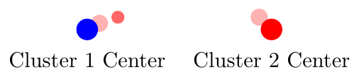
Soft clustering assigns each data point a probability or degree of membership to multiple clusters simultaneously. This allows data points to partially belong to several groups.
Example: A data point may have a 70% membership in Cluster 1 and 30% in Cluster 2.
Use Cases: Situations with overlapping boundaries, fuzzy categories, customer personas, or medical diagnosis.
Benefits: Captures ambiguity, models gradual transitions between clusters.
Types of Clustering Methods
Clustering methods can be classified based on how they form clusters:
1. Centroid-based Clustering (Partitioning Methods)
Organizes data points around centroids (mean or medoid).
Algorithms:
K-means: minimizes intra-cluster variance.
K-medoids: uses actual data points, robust to outliers.
Advantages: Fast, scalable, easy to implement.
Limitations: Requires number of clusters, sensitive to outliers, not suitable for non-spherical clusters.
2. Density-based Clustering (Model-based Methods)
Forms clusters as high-density regions separated by low-density areas.
Algorithms:
DBSCAN: identifies clusters and noise.
OPTICS: handles varying density clusters.
Advantages: Detects arbitrary shapes, handles noise, cluster count not required.
Limitations: Parameter selection can be difficult, less effective for varying densities (except OPTICS).
3. Connectivity-based Clustering (Hierarchical Clustering)
Builds nested clusters based on connectivity among points.
Approaches:
Agglomerative (Bottom-up): merge closest clusters iteratively.
Divisive (Top-down): split clusters iteratively.
Advantages: Full hierarchy, easy visualization, cluster count not needed.
Limitations: Computationally expensive, merging/splitting decisions are irreversible.
4. Distribution-based Clustering
Assumes data comes from a mixture of probability distributions.
Algorithm: Gaussian Mixture Model (GMM): assigns points based on likelihood.
Advantages: Flexible cluster shapes, probabilistic memberships, handles overlapping clusters.
Limitations: Requires number of components, computationally expensive, sensitive to initialization.
5. Fuzzy Clustering
Allows points to belong to multiple clusters with degrees of membership.
Algorithm: Fuzzy C-Means: updates fuzzy memberships iteratively.
Advantages: Captures ambiguity, suitable for overlapping clusters.
Limitations: Choosing fuzziness parameter can be tricky, higher computational cost.
Partition-based Clustering
Partition-based clustering algorithms divide the dataset into a predefined number of clusters $k$, optimizing a cluster-specific objective function. They are widely used because of their simplicity and efficiency, especially for large datasets. The most common algorithms are K-means and K-medoids.
K-means Clustering
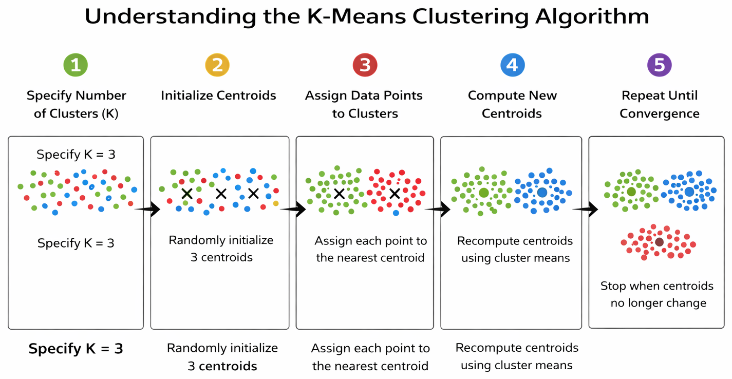
Step 1: Specify Number of Clusters
Let the dataset be \[ \mathcal{D} = \{x_1, x_2, \ldots, x_n\}, \quad x_i \in \mathbb{R}^d \]
Fix the number of clusters: \[ K \in \mathbb{N} \]
Step 2: Initialize Centroids Randomly
Select \(K\) distinct data points as initial centroids: \[ \mu_1^{(0)}, \mu_2^{(0)}, \ldots, \mu_K^{(0)} \in \mathcal{D} \]
Step 3: Distance Computation & Assignment Step (Cluster Membership)
For each data point \(x_i\), compute the squared Euclidean distance to all centroids and assign it to the nearest one: \[ c_i^{(t)} = \arg\min_{k \in \{1,\ldots,K\}} \|x_i - \mu_k^{(t)}\|_2^2 \]
Thus, \[ x_i \in C_k^{(t)} \quad \text{if } c_i^{(t)} = k \]
Step 4: Update Step (Centroid Recalculation)
Recompute each centroid as the mean of the data points assigned to that cluster: \[ \mu_k^{(t+1)} = \frac{1}{|C_k^{(t)}|} \sum_{x_i \in C_k^{(t)}} x_i \]
Step 5: Stopping Criterion (Convergence)
Iterate Steps 3–4 until convergence, i.e., stop if either: \[ C_k^{(t+1)} = C_k^{(t)} \quad \forall k \]
or \[ \mu_k^{(t+1)} = \mu_k^{(t)} \quad \forall k \]
Given a dataset in $\mathbb{R}^2$, \[ D = \left\{ x_1 = (1,1),\; x_2 = (1,2),\; x_3 = (4,4),\; x_4 = (5,4) \right\}, \] apply the K-means clustering algorithm with \[ K = 2 \] clusters. Perform the algorithm step by step until convergence.
—
Step 1: Specify Number of Clusters
\[ K = 2 \]
—
Step 2: Initialize Centroids
Choose two data points as initial centroids: \[ \mu_1^{(0)} = (1,1), \qquad \mu_2^{(0)} = (5,4) \]
—
Step 3: Distance Computation and Assignment
The squared Euclidean distance is given by \[ \|x - \mu\|^2 = (x_1 - \mu_1)^2 + (x_2 - \mu_2)^2 \]
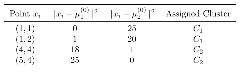
\[ C_1^{(0)} = \{(1,1),(1,2)\}, \qquad C_2^{(0)} = \{(4,4),(5,4)\} \]
—
Step 4: Update Step (Centroid Recalculation)
Compute the new centroids as the mean of points in each cluster.
\[ \mu_1^{(1)} = \frac{(1,1) + (1,2)}{2} = (1,1.5) \]
\[ \mu_2^{(1)} = \frac{(4,4) + (5,4)}{2} = (4.5,4) \]
—
Step 5: Reassignment Using Updated Centroids
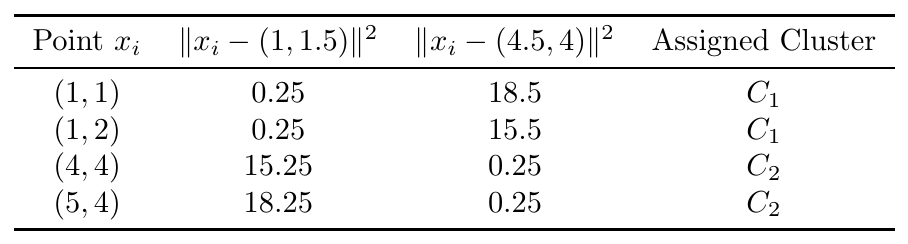
Since the cluster assignments do not change, the algorithm converges.
—
Final Result
Clusters \[ C_1 = \{(1,1),(1,2)\}, \qquad C_2 = \{(4,4),(5,4)\} \]
Centroids \[ \mu_1 = (1,1.5), \qquad \mu_2 = (4.5,4) \]
$\blacksquare$
Advantages: Simple, scalable, efficient for large datasets.
Limitations: Sensitive to initialization, outliers, assumes spherical clusters, requires pre-defined $k$.
K-medoids Clustering
K-medoids clustering is similar to K-means but uses actual data points as cluster centers (medoids) instead of the mean. This makes it robust to outliers.
Steps:
Initialize $k$ medoids randomly from data points.
Assign each point to the nearest medoid.
For each cluster, try swapping medoid with another point in cluster; if total cost decreases, update medoid.
Repeat step 3 until no improvement.
Step 1: Specify Number of Clusters
Let the dataset be \[ \mathcal{D} = \{x_1, x_2, \ldots, x_n\}, \quad x_i \in \mathbb{R}^d \]
Fix the number of clusters: \[ K \in \mathbb{N} \]
—
Step 2: Initialize Medoids Randomly
Select \(K\) distinct data points as initial medoids: \[ m_1^{(0)}, m_2^{(0)}, \ldots, m_K^{(0)} \in \mathcal{D} \]
Each \(m_k\) is a representative data point of cluster \(C_k\).
—
Step 3: Distance Computation & Assignment Step
Assign each data point to the nearest medoid using a distance metric: \[ c_i^{(t)} = \arg\min_{k \in \{1,\ldots,K\}} \text{dist}(x_i, m_k^{(t)}) \]
Thus, \[ x_i \in C_k^{(t)} \quad \text{if } c_i^{(t)} = k \]
—
Step 4: Update Step (Medoid Recalculation)
For each cluster \(C_k^{(t)}\), choose the new medoid as the data point that minimizes the total distance to all other points in that cluster: \[ m_k^{(t+1)} = \arg\min_{x_j \in C_k^{(t)}} \sum_{x_i \in C_k^{(t)}} \text{dist}(x_i, x_j) \]
—
Step 5: Stopping Criterion (Convergence)
Iterate Steps 3–4 until convergence, i.e., stop if: \[ m_k^{(t+1)} = m_k^{(t)} \quad \forall k \] or cluster assignments do not change.
—
Objective Function
K-medoids minimizes the total within-cluster dissimilarity: \[ \boxed{ \sum_{k=1}^{K} \sum_{x_i \in C_k} \text{dist}(x_i, m_k) } \]
Unlike K-means, the distance need not be squared and can be any valid metric.
Given Dataset
\[ \mathcal{D} = \{1, 2, 4, 10\}, \quad K = 2 \]
—
Initialization
Choose initial medoids: \[ m_1^{(0)} = 1, \qquad m_2^{(0)} = 10 \]
—
Assignment Step
Using absolute distance:
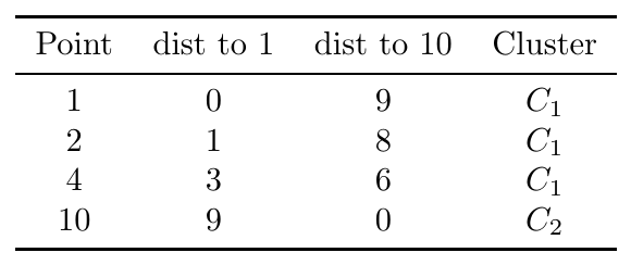
\[ C_1 = \{1,2,4\}, \quad C_2 = \{10\} \]
—
Medoid Update
Compute total distances within \(C_1\):
\[ \begin{aligned} \text{cost}(1) &= |1-1| + |2-1| + |4-1| = 4 \\ \text{cost}(2) &= |1-2| + |2-2| + |4-2| = 3 \\ \text{cost}(4) &= |1-4| + |2-4| + |4-4| = 5 \end{aligned} \]
Thus, the new medoid is: \[ m_1^{(1)} = 2 \]
For cluster \(C_2\): \[ m_2^{(1)} = 10 \]
—
Convergence
Medoids change from \((1,10)\) to \((2,10)\). Reassignment does not change the clusters; hence the algorithm converges.
—
Final Result
Clusters \[ C_1 = \{1,2,4\}, \quad C_2 = \{10\} \]
Medoids \[ m_1 = 2, \quad m_2 = 10 \]
$\blacksquare$
K-means uses mean, sensitive to outliers; K-medoids uses medoid, robust to outliers.
K-means is faster (simple arithmetic mean), K-medoids is computationally expensive (pairwise distances).
Both require pre-defined $k$.
Hierarchical Clustering
Hierarchical clustering is an unsupervised learning technique that seeks to build a hierarchy of clusters. Unlike K-means, it does not require a pre-specified number of clusters. Hierarchical clustering can be agglomerative (bottom-up) or divisive (top-down).
Agglomerative (Bottom-Up) Approach
Agglomerative clustering starts with each point as a singleton cluster and iteratively merges the two closest clusters until a stopping criterion is met (e.g., all points in one cluster or a threshold distance).
Algorithm: Bottom-Up (Agglomerative) Hierarchical Clustering
Initialization: Start with each data point as its own cluster: \[ C_i = \{x_i\}, \quad i = 1,2,\dots,n \]
Compute Distance Matrix: Compute all pairwise distances between clusters using a chosen metric (e.g., Euclidean distance): \[ d(C_i, C_j) = \min/\max/\text{average}_{x \in C_i, y \in C_j} d(x,y) \] depending on the linkage criterion (single, complete, or average).
Merge Clusters: Identify the pair of clusters with the minimum distance according to the chosen linkage criterion and merge them.
Update Distances: Recompute distances between the new cluster and all remaining clusters using the linkage criterion.
Stopping Criterion: Repeat Steps 3–4 until one of the following conditions is met:
Desired number of clusters is reached.
Only a single cluster remains (complete hierarchy formed).
The key step is defining the inter-cluster distance. Two popular methods are:
Single-Linkage Method
Definition: The distance between two clusters $A$ and $B$ is the minimum distance between any two points in the clusters:
\[ D_{\text{single}}(A,B) = \min_{x \in A, y \in B} \|x-y\| \]
Characteristics:
Can produce elongated, chain-like clusters.
Sensitive to noise and outliers.
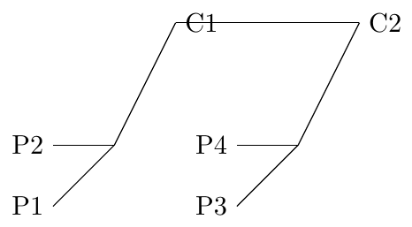
Consider points on a 2D plane: $P_1=(1,1), P_2=(2,1), P_3=(5,5), P_4=(6,5)$. Perform single-linkage clustering.
Solution:
Compute all pairwise distances: $P_1-P_2=1$, $P_1-P_3 \approx 5.66$, $P_1-P_4 \approx 6.40$, $P_2-P_3 \approx 5.0$, $P_2-P_4 \approx 5.83$, $P_3-P_4=1$.
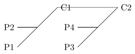
Merge closest pair $P_1$ and $P_2$ → Cluster $C_1 = \{P_1,P_2\}$. Merge closest remaining pair $P_3$ and $P_4$ → Cluster $C_2 = \{P_3,P_4\}$.
Compute inter-cluster distance $D_{\text{single}}(C_1,C_2) = \min\{\|P_1-P_3\|, \|P_1-P_4\|, \|P_2-P_3\|, \|P_2-P_4\|\} = 5.0$.
Merge $C_1$ and $C_2$ if required.
Dendrogram:
Complete/Multiple-Linkage Method
Definition: The distance between two clusters $A$ and $B$ is the maximum distance between any two points in the clusters:
\[ D_{\text{complete}}(A,B) = \max_{x \in A, y \in B} \|x-y\| \]
Characteristics:
Produces compact, spherical clusters.
Less sensitive to outliers compared to single-linkage.
Using the same points as above: $P_1=(1,1), P_2=(2,1), P_3=(5,5), P_4=(6,5)$, perform complete-linkage clustering.
Solution:
Merge closest pair $P_1$ and $P_2$ → Cluster $C_1=\{P_1,P_2\}$, and $P_3$ and $P_4$ → $C_2=\{P_3,P_4\}$.
Compute inter-cluster distance $D_{\text{complete}}(C_1,C_2) = \max\{\|P_1-P_3\|, \|P_1-P_4\|, \|P_2-P_3\|, \|P_2-P_4\|\} = 6.40$.
Merge only if threshold allows.
Dendrogram: (Shows complete linkage produces slightly higher linkage height)
Example: Bottom-Up (Agglomerative) Hierarchical Clustering
Consider the one-dimensional dataset: \[ D = \{x_1=1,\, x_2=2,\, x_3=5,\, x_4=6\} \] with Euclidean distance \[ d(x_i, x_j) = |x_i - x_j|. \]
Initially, each point is a separate cluster: \[ C_1 = \{1\},\; C_2 = \{2\},\; C_3 = \{5\},\; C_4 = \{6\}. \]
Step 1: Compute Pairwise Distance Matrix
\[ \begin{array}{c|cccc} & 1 & 2 & 5 & 6 \\ \hline 1 & 0 & 1 & 4 & 5 \\ 2 & 1 & 0 & 3 & 4 \\ 5 & 4 & 3 & 0 & 1 \\ 6 & 5 & 4 & 1 & 0 \end{array} \]
Step 2: Single Linkage Clustering
Merge the two clusters with minimum distance. Minimum distance = 1, merge $C_1$ and $C_2$: \[ C_{12} = \{1,2\} \] Remaining clusters: $C_{12}, C_3, C_4$
Next minimum distance = 1, merge $C_3$ and $C_4$: \[ C_{34} = \{5,6\} \]
Distance between $C_{12}$ and $C_{34}$ (single linkage): \[ d_{\text{single}}(C_{12}, C_{34}) = \min\{3,4,4,5\} = 3 \] Merge to form final cluster $C_{1234} = \{1,2,5,6\}$
Step 3: Complete Linkage Clustering
Merge $C_1$ and $C_2$, $C_{12} = \{1,2\}$
Merge $C_3$ and $C_4$, $C_{34} = \{5,6\}$
Distance between $C_{12}$ and $C_{34}$ (complete linkage): \[ d_{\text{complete}}(C_{12}, C_{34}) = \max\{4,5,3,4\} = 5 \] Merge to form final cluster $C_{1234} = \{1,2,5,6\}$
Step 4: Average Linkage Clustering
Merge $C_1$ and $C_2$, $C_{12} = \{1,2\}$
Merge $C_3$ and $C_4$, $C_{34} = \{5,6\}$
Distance between $C_{12}$ and $C_{34}$ (average linkage): \[ d_{\text{avg}}(C_{12}, C_{34}) = \frac{4+5+3+4}{4} = 4 \] Merge to form final cluster $C_{1234} = \{1,2,5,6\}$
Step 5: Observations
Single linkage produces chained, elongated clusters.
Complete linkage produces compact clusters.
Average linkage gives a balanced clustering.
Divisive (Top-Down) Approach
Definition: Divisive clustering starts with all points in a single cluster and recursively splits clusters into smaller sub-clusters until each point forms its own cluster or a stopping criterion is satisfied.
Procedure:
Start with the full dataset as a single cluster.
Select a cluster to split based on a criterion (e.g., maximize intra-cluster distance or minimize inter-cluster similarity).
Split the selected cluster into two sub-clusters. This can be done using methods such as:
K-means or K-medoids on the cluster to partition it into two groups.
Principal Component Analysis (PCA) to find the direction of maximum variance and split along it.
Repeat steps 2–3 recursively on the new clusters until stopping criteria are met (e.g., desired number of clusters, minimal cluster size, or distance threshold).
Distance Measure: For splitting, a common choice is the diameter of the cluster: \[ \text{diameter}(C) = \max_{x_i, x_j \in C} \|x_i - x_j\| \] Clusters with larger diameter are often chosen first to split.
Characteristics:
Produces a hierarchy of clusters similar to agglomerative clustering but in reverse order.
Computationally more expensive than agglomerative methods for large datasets.
Flexible in choosing splitting criteria and distance measures.
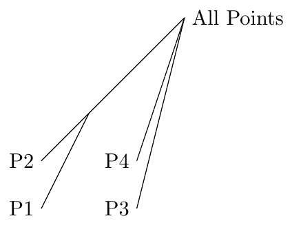
Consider points $P_1=(1,1), P_2=(2,1), P_3=(5,5), P_4=(6,5)$.
Start with cluster $C = \{P_1,P_2,P_3,P_4\}$.
Compute the pairwise distances and find the two points with maximum dissimilarity. Here, $\|P_1-P_4\| = 6.40$.
Split the cluster into $C_1 = \{P_1,P_2\}$ and $C_2 = \{P_3,P_4\}$.
Recursively apply the same procedure if more splits are required.
Dendrogram:
Comparison:
Agglomerative is bottom-up, divisive is top-down.
Agglomerative is more commonly used in practice.
Choice of linkage affects cluster shape and sensitivity to noise.
Example: Divisive (Top-Down) Hierarchical Clustering
Consider the one-dimensional dataset: \[ D = \{1, 2, 5, 6\} \] with Euclidean distance: \[ d(x_i, x_j) = |x_i - x_j|. \]
Step 1: Start with a single cluster
\[ C^{(0)} = \{1, 2, 5, 6\} \]
Step 2: Identify cluster to split
- Only one cluster exists. - Compute cluster diameter: \[ \text{diameter}(C^{(0)}) = \max(D) - \min(D) = 6 - 1 = 5 \]
Step 3: Split the cluster
- Use $k$-means with $K=2$ to divide the cluster:
\[ C_1 = \{1,2\}, \quad C_2 = \{5,6\} \]
- Compute cluster centroids: \[ \mu_1 = \frac{1+2}{2} = 1.5, \quad \mu_2 = \frac{5+6}{2} = 5.5 \]
Step 4: Update clusters
\[ C_1 = \{1,2\}, \quad C_2 = \{5,6\} \]
Step 5: Stopping criterion
- Desired number of clusters ($K=2$) is reached, so stop.
Final Result
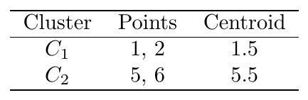
Observation: Divisive clustering works top-down, splitting large clusters recursively. Linkage criteria are not used, unlike in agglomerative clustering.