Dimensionality Reduction
Principal Component Analysis (PCA)
Introduction and Motivation
Dimensionality reduction is crucial in machine learning when dealing with high-dimensional datasets. High dimensions lead to several challenges:
Curse of dimensionality: Distances become less meaningful as dimensionality increases.
Visualization: Difficult to visualize data beyond 3 dimensions.
Computational cost: More features mean more computation in ML models.
Redundancy: Many features are correlated and carry overlapping information.
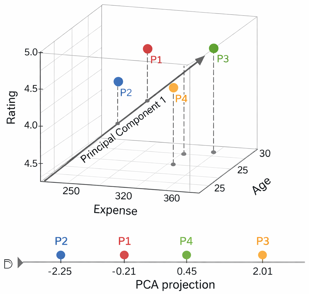
Idea: PCA transforms the original correlated features into a smaller set of uncorrelated variables called principal components (PCs) while retaining most of the variance in the data.
Benefits:
Reduces dimensionality and computational cost.
Removes feature correlations.
Preserves maximum variance.
Visualization of PCA Projection
Mathematical Formulation
Setup Assuming population data:
Let there be $n$ data points and $d$ features.
\[ X = \begin{bmatrix} x_{11} & x_{12} & \cdots & x_{1d} \\ x_{21} & x_{22} & \cdots & x_{2d} \\ \vdots & \vdots & \ddots & \vdots \\ x_{n1} & x_{n2} & \cdots & x_{nd} \end{bmatrix} \in \mathbb{R}^{n \times d} \]
Here, \[ i = 1,\dots,n \quad (\text{samples}), \qquad j = 1,\dots,d \quad (\text{features}) \]
—
Step 1: Data Standardization (Zero Mean, Unit Variance)
Mean of feature $j$: \[ \mu_j = \frac{1}{n} \sum_{i=1}^{n} x_{ij} \]
Standard deviation of feature $j$: \[ \sigma_j = \sqrt{\frac{1}{n} \sum_{i=1}^{n} (x_{ij} - \mu_j)^2} \]
Standardized data: \[ z_{ij} = \frac{x_{ij} - \mu_j}{\sigma_j} \]
—
Step 2: Standardized Data Matrix
\[ Z = \begin{bmatrix} z_{11} & z_{12} & \cdots & z_{1d} \\ z_{21} & z_{22} & \cdots & z_{2d} \\ \vdots & \vdots & \ddots & \vdots \\ z_{n1} & z_{n2} & \cdots & z_{nd} \end{bmatrix} \in \mathbb{R}^{n \times d} \]
—
Step 3: Covariance Matrix
\[ C = \frac{1}{n} Z^{T} Z \quad \in \mathbb{R}^{d \times d} \]
Properties: \[ C = C^T \quad (\text{symmetric}) \] \[ \lambda_i \ge 0 \quad (\text{positive semi-definite}) \]
—
Step 4: Eigenvalues and Eigenvectors
Solve: \[ |C - \lambda I| = 0 \]
\[ C v_i = \lambda_i v_i \]
Eigenvalues ordered as: \[ \lambda_1 \ge \lambda_2 \ge \cdots \ge \lambda_d \ge 0 \]
Interpretation: \[ \lambda_i \rightarrow \text{variance along direction } v_i \] \[ v_i \rightarrow \text{principal axis} \]
—
Step 5: Selection of Principal Components
Choose top $k$ eigenvectors corresponding to largest eigenvalues.
\[ W = [v_1 \; v_2 \; \cdots \; v_k] \in \mathbb{R}^{d \times k} \]
Explained variance ratio: \[ \text{Variance explained by } \lambda_i = \frac{\lambda_i}{\sum_{j=1}^{d} \lambda_j} \]
—
Step 6: Projection (Dimensionality Reduction)
\[ Y = Z W \]
\[ Y \in \mathbb{R}^{n \times k} \]
This gives the representation of data in the new principal component space.
Principal components are orthogonal.
First PC captures maximum variance.
Total variance in data = sum of eigenvalues.
Fraction of variance captured by $i$-th PC: $\lambda_i / \sum_j \lambda_j$
Given Data
\[ X = \begin{bmatrix} 2 & 0 \\ 0 & 1 \\ 3 & 1 \\ 4 & 3 \end{bmatrix} \in \mathbb{R}^{4 \times 2} \]
Here, $n = 4$ samples and $d = 2$ features.
—
Step 1: Compute Mean and Standard Deviation
Mean of each feature: \[ \mu_1 = \frac{2+0+3+4}{4} = 2.25, \quad \mu_2 = \frac{0+1+1+3}{4} = 1.25 \]
Standard deviation: \[ \sigma_1 = \sqrt{\frac{1}{4}\left[(2-2.25)^2 + (0-2.25)^2 + (3-2.25)^2 + (4-2.25)^2\right]} = 1.479 \]
\[ \sigma_2 = \sqrt{\frac{1}{4}\left[(0-1.25)^2 + (1-1.25)^2 + (1-1.25)^2 + (3-1.25)^2\right]} = 1.090 \]
—
Step 2: Standardization
\[ z_{ij} = \frac{x_{ij} - \mu_j}{\sigma_j} \]
\[ Z = \begin{bmatrix} -0.17 & -1.15 \\ -1.52 & -0.23 \\ 0.51 & -0.23 \\ 1.18 & 1.61 \end{bmatrix} \in \mathbb{R}^{4 \times 2} \]
—
Step 3: Covariance Matrix
\[ C = \frac{1}{n} Z^T Z \]
\[ C = \begin{bmatrix} 1.00 & 0.69 \\ 0.69 & 1.00 \end{bmatrix} \]
—
Step 4: Eigenvalues and Eigenvectors
\[ |C - \lambda I| = 0 \]
\[ \lambda_1 = 1.69, \quad \lambda_2 = 0.31 \]
Corresponding eigenvectors: \[ v_1 = \frac{1}{\sqrt{2}} \begin{bmatrix} 1 \\ 1 \end{bmatrix}, \quad v_2 = \frac{1}{\sqrt{2}} \begin{bmatrix} 1 \\ -1 \end{bmatrix} \]
—
Step 5: Selection of Principal Component
\[ \frac{\lambda_1}{\lambda_1 + \lambda_2} = \frac{1.69}{2} = 84.5\% \]
Select $k = 1$ principal component.
\[ W = v_1 = \frac{1}{\sqrt{2}} \begin{bmatrix} 1 \\ 1 \end{bmatrix} \]
—
Step 6: Projection
\[ Y = Z W \]
\[ Y = \begin{bmatrix} -0.93 \\ -1.23 \\ 0.20 \\ 1.96 \end{bmatrix} \in \mathbb{R}^{4 \times 1} \]
—
Final Result
The original 2D data is reduced to 1D while preserving maximum variance.
Given Data
\[ X = \begin{bmatrix} 2 & 2 & 3 \\ 3 & 3 & 4 \\ 4 & 4 & 5 \\ 5 & 5 & 6 \end{bmatrix} \in \mathbb{R}^{4 \times 3} \]
The three features $X_1, X_2, X_3$ are highly correlated.
—
Step 1: Standardization (Mean Centering)
Compute the mean of each feature: \[ \mu = \begin{bmatrix} 3.5 & 3.5 & 4.5 \end{bmatrix} \]
Centered data matrix: \[ Z = X - \mu = \begin{bmatrix} -1.5 & -1.5 & -1.5 \\ -0.5 & -0.5 & -0.5 \\ 0.5 & 0.5 & 0.5 \\ 1.5 & 1.5 & 1.5 \end{bmatrix} \]
—
Step 2: Covariance Matrix
\[ C = \frac{1}{n} Z^T Z \]
Since all features move together, the covariance matrix has large off-diagonal entries: \[ C = \begin{bmatrix} \sigma^2 & \sigma^2 & \sigma^2 \\ \sigma^2 & \sigma^2 & \sigma^2 \\ \sigma^2 & \sigma^2 & \sigma^2 \end{bmatrix} \]
This indicates strong positive correlation among $X_1, X_2, X_3$.
—
Step 3: Eigenvalue Decomposition
Solve: \[ C v = \lambda v \]
The dominant eigenvector is: \[ v_1 = \frac{1}{\sqrt{3}} \begin{bmatrix} 1 \\ 1 \\ 1 \end{bmatrix} \]
This direction captures maximum variance.
Remaining eigenvectors are orthogonal to $v_1$ and correspond to very small eigenvalues, capturing negligible variance.
—
Interpretation
\[ \lambda_1 \gg \lambda_2, \lambda_3 \]
Most of the variance lies along the direction $(1,1,1)$.
Therefore, the original 3D data can be projected onto a single principal component:
\[ Y = Z v_1 \]
This reduces the data from $\mathbb{R}^3$ to $\mathbb{R}^1$ while preserving most of the information.
—
Conclusion
PCA effectively reduces the dimensionality from 3 to 1 due to high correlation among features.