Vector Spaces
Vectors Concept
What is a Vector?
A vector is a mathematical object that has both magnitude and direction. In coordinate form, a vector in $\R^n$ is an ordered tuple \[ \mathbf{v} = (v_1, v_2, \dots, v_n) \in \R^n. \] Vectors are usually written in bold (e.g. \(\mathbf{v}\)) or with an arrow overhead (\(\vec{v}\)). A zero vector has all components zero and is denoted \(\mathbf{0}\).
Geometric picture and basic diagrams
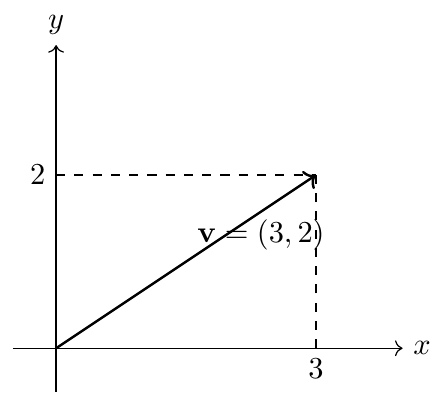
A vector in 2D can be drawn as a directed arrow from the origin to the point $(x,y)$. Vectors can be translated (moved) without changing their meaning as long as direction and magnitude remain same.
Length or Magnitude of a Vector
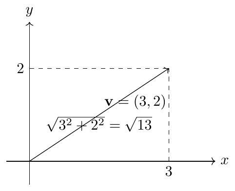
The length (or magnitude or norm) of a vector $\mathbf{v}$ represents how long the vector is — that is, its distance from the origin to the point it represents in space.
If $\mathbf{v} = (v_1, v_2, v_3, \dots, v_n)$ in $\mathbb{R}^n$, then the magnitude of $\mathbf{v}$ is given by \[ \norm{\mathbf{v}} = \sqrt{v_1^2 + v_2^2 + v_3^2 + \dots + v_n^2}. \]
This follows from the **Pythagorean theorem** generalized to $n$ dimensions.
Properties:
$\norm{\mathbf{v}} \ge 0$ for all vectors.
$\norm{\mathbf{v}} = 0 \iff \mathbf{v} = \mathbf{0}$.
$\norm{k\mathbf{v}} = |k|\norm{\mathbf{v}}$ for any scalar $k$.
The distance between two points $\mathbf{A}$ and $\mathbf{B}$ is $\norm{\mathbf{A} - \mathbf{B}}$.
For $\mathbf{v} = (3,4)$, \[ \norm{\mathbf{v}} = \sqrt{3^2 + 4^2} = 5. \]
For $\mathbf{v} = (1,2,2)$, \[ \norm{\mathbf{v}} = \sqrt{1^2 + 2^2 + 2^2} = 3. \]
Let $A(1,2,3)$ and $B(4,6,9)$. Then vector $\overrightarrow{AB} = B - A = (3,4,6)$, and \[ \text{Distance } = \norm{\overrightarrow{AB}} = \sqrt{3^2 + 4^2 + 6^2} = \sqrt{61}. \]
Let \(\mathbf{a}=(3,-1,2)\). Then $\mathbf{a}$ is a vector in $\R^3$ with magnitude \[ \norm{\mathbf{a}} = \sqrt{3^2 + (-1)^2 + 2^2} = \sqrt{14}. \]
Vector arithmetic
Given $\mathbf{u}=(u_1,\dots,u_n)$ and $\mathbf{v}=(v_1,\dots,v_n)$ in $\R^n$ and scalar $\alpha\in\R$:
Addition: \(\mathbf{u}+\mathbf{v}=(u_1+v_1,\dots,u_n+v_n)\).
Scalar multiplication: \(\alpha\mathbf{v}=(\alpha v_1,\dots,\alpha v_n)\).
Subtraction: \(\mathbf{u}-\mathbf{v}=(u_1-v_1,\dots,u_n-v_n)\).
Vector operations satisfy commutativity, associativity, distributivity, existence of zero vector and additive inverses.
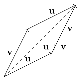
Let $\mathbf{u}=(1,2)$ and $\mathbf{v}=(3,-1)$. Then \[ \mathbf{u}+\mathbf{v}=(4,1),\qquad 2\mathbf{u}=(2,4). \] Geometric interpretation: addition corresponds to placing vectors head-to-tail (parallelogram rule).
Dot product (Inner product) and properties
For $\mathbf{u},\mathbf{v}\in\R^n$, the dot product (inner product) is \[ \mathbf{u}\cdot\mathbf{v} = \sum_{i=1}^n u_i v_i. \] Properties:
Symmetry: $\mathbf{u}\cdot\mathbf{v}=\mathbf{v}\cdot\mathbf{u}$.
Linearity: $(a\mathbf{u}+b\mathbf{w})\cdot\mathbf{v} = a(\mathbf{u}\cdot\mathbf{v}) + b(\mathbf{w}\cdot\mathbf{v})$.
Positive-definiteness: $\mathbf{v}\cdot\mathbf{v}=\norm{\mathbf{v}}^2 \ge 0$ and equals zero only for $\mathbf{v}=\mathbf{0}$.
Relation to angle: $\mathbf{u}\cdot\mathbf{v} = \norm{\mathbf{u}}\norm{\mathbf{v}} \cos\theta$, where $\theta$ is the angle between them.
Let $\mathbf{a}=(1,1,0)$ and $\mathbf{b}=(1,0,1)$. Then \[ \mathbf{a}\cdot\mathbf{b}=1\cdot1+1\cdot0+0\cdot1=1, \] \[ \norm{\mathbf{a}}=\sqrt{2},\quad \norm{\mathbf{b}}=\sqrt{2}\quad\Rightarrow\quad \cos\theta=\frac{1}{2}. \] So $\theta = \cos^{-1}\left(\tfrac{1}{2}\right)=60^\circ$.
Norms and distances
The (Euclidean) norm of $\mathbf{v}\in\R^n$ is $\norm{\mathbf{v}}=\sqrt{\mathbf{v}\cdot\mathbf{v}}$. Distance between points $\mathbf{p},\mathbf{q}\in\R^n$ is $\norm{\mathbf{p}-\mathbf{q}}$.
Triangle inequality: \[ \norm{\mathbf{u}+\mathbf{v}} \le \norm{\mathbf{u}} + \norm{\mathbf{v}}. \] Cauchy–Schwarz inequality: \[ |\mathbf{u}\cdot\mathbf{v}| \le \norm{\mathbf{u}}\,\norm{\mathbf{v}}. \]
Take $\mathbf{u}=(1,0)$ and $\mathbf{v}=(0,1)$. Then $\norm{\mathbf{u}}=\norm{\mathbf{v}}=1$ and $\norm{\mathbf{u}+\mathbf{v}}=\sqrt{2}\le 2$ holds.
Cross product (3D) and properties
For $\mathbf{a},\mathbf{b}\in\R^3$, the cross product $\mathbf{a}\times\mathbf{b}$ is a vector perpendicular to both, given by the determinant formula: \[ \mathbf{a}\times\mathbf{b} = \begin{vmatrix} \mathbf{i} & \mathbf{j} & \mathbf{k} \\ a_1 & a_2 & a_3 \\ b_1 & b_2 & b_3 \end{vmatrix}. \] Properties:
$\mathbf{a}\times\mathbf{b} = -(\mathbf{b}\times\mathbf{a})$ (antisymmetric).
$\norm{\mathbf{a}\times\mathbf{b}} = \norm{\mathbf{a}}\norm{\mathbf{b}}\sin\theta$ (area of parallelogram).
$(\mathbf{a}\times\mathbf{b})\cdot\mathbf{a}=0$ and $(\mathbf{a}\times\mathbf{b})\cdot\mathbf{b}=0$.
Cross product is defined only in 3D (or via wedge product in higher dimensional algebra).
Let $\mathbf{a}=(1,0,0)$ and $\mathbf{b}=(0,1,0)$. Then $\mathbf{a}\times\mathbf{b}=(0,0,1)$.
Triangle with vertices $A(1,0,0)$, $B(2,1,0)$, $C(1,1,1)$. Area = $\tfrac12 \norm{(\overrightarrow{AB}\times\overrightarrow{AC})}$. Compute $\overrightarrow{AB}=(1,1,0)$, $\overrightarrow{AC}=(0,1,1)$. \[ \overrightarrow{AB}\times\overrightarrow{AC} = \begin{vmatrix} \mathbf{i} & \mathbf{j} & \mathbf{k} \\ 1 & 1 & 0 \\ 0 & 1 & 1 \end{vmatrix} = (1\cdot1-0\cdot1)\mathbf{i} - (1\cdot1-0\cdot0)\mathbf{j} + (1\cdot1-1\cdot0)\mathbf{k} = (1,-1,1). \] Norm $=\sqrt{3}$, area $=\tfrac12\sqrt{3}$.
Vector Space
Elimination simplifies the system $A\mathbf{x} = \mathbf{b}$, one entry at a time. It also simplifies the underlying theory — particularly the fundamental questions of **existence** and **uniqueness** of solutions:
Does the system have one unique solution?
Does it have no solution?
Or does it have infinitely many solutions?
After elimination, these questions become easier to answer. However, elimination gives only one kind of understanding of $A\mathbf{x} = \mathbf{b}$. Linear algebra goes deeper — it explores the very structure of the space that these vectors and equations belong to.
Concept of a Vector Space
To develop a deeper understanding, we begin with the most fundamental spaces, denoted by: \[ \mathbb{R}^1, \ \mathbb{R}^2, \ \mathbb{R}^3, \dots, \mathbb{R}^n \] Each $\mathbb{R}^n$ consists of all column vectors with $n$ real components.
$\mathbb{R}^1$ — all real numbers (a line)
$\mathbb{R}^2$ — the usual $xy$-plane
$\mathbb{R}^3$ — three-dimensional space
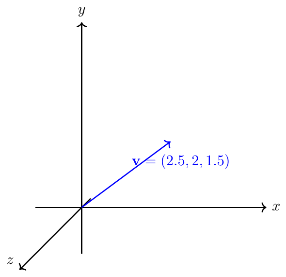
The two components of a vector in $\mathbb{R}^2$ represent the $x$ and $y$ coordinates of a point in the plane. Similarly, the three components of a vector in $\mathbb{R}^3$ represent a point in three-dimensional space.
Generalization to Higher Dimensions
The beauty of linear algebra lies in how naturally it extends to higher dimensions. A vector in $\mathbb{R}^7$, for example, is represented simply by its seven components: \[ \mathbf{x} = (x_1, x_2, x_3, x_4, x_5, x_6, x_7) \] Even though we cannot visualize 7-dimensional geometry, all algebraic operations remain the same:
Vector addition: $\mathbf{x} + \mathbf{y}$
Scalar multiplication: $c\mathbf{x}$
Definition of a Real Vector Space
A real vector space is a set of elements (vectors) together with two operations:
Vector addition
Scalar multiplication by real numbers
These operations must:
Produce vectors that remain inside the space.
Satisfy the eight basic vector space axioms.
Eight Basic Axioms of Vector Spaces
Closure under addition: For all \( \mathbf{u}, \mathbf{v} \in V \), the sum \( \mathbf{u} + \mathbf{v} \in V \).
Commutative property of addition: \( \mathbf{u} + \mathbf{v} = \mathbf{v} + \mathbf{u} \).
Associative property of addition: \( (\mathbf{u} + \mathbf{v}) + \mathbf{w} = \mathbf{u} + (\mathbf{v} + \mathbf{w}) \).
Existence of additive identity: There exists a zero vector \( \mathbf{0} \in V \) such that \( \mathbf{v} + \mathbf{0} = \mathbf{v} \).
Existence of additive inverse: For every \( \mathbf{v} \in V \), there exists \( -\mathbf{v} \in V \) such that \( \mathbf{v} + (-\mathbf{v}) = \mathbf{0} \).
Closure under scalar multiplication: For all \( c \in \mathbb{R} \) and \( \mathbf{v} \in V \), \( c\mathbf{v} \in V \).
Distributive laws: \begin{align*} c(\mathbf{u} + \mathbf{v}) &= c\mathbf{u} + c\mathbf{v} &(scalar over vector addition)
(c + d)\mathbf{v} &= c\mathbf{v} + d\mathbf{v} &(scalar addition over vector) \end{align*}Compatibility with scalar multiplication: \( c(d\mathbf{v}) = (cd)\mathbf{v} \) and \( 1\mathbf{v} = \mathbf{v} \).
Let \( V = \mathbb{R}^2 = \{ (x, y) \mid x, y \in \mathbb{R} \} \). Define addition and scalar multiplication as: \[ (x_1, y_1) + (x_2, y_2) = (x_1 + x_2, \, y_1 + y_2), \quad c(x, y) = (cx, cy) \]
Let us verify some axioms:
Closure under addition: If \( (x_1, y_1), (x_2, y_2) \in \mathbb{R}^2 \), then \( (x_1 + x_2, y_1 + y_2) \in \mathbb{R}^2 \).
Existence of additive identity: \( (0,0) \) is the zero vector since \( (x,y) + (0,0) = (x,y) \).
Existence of additive inverse: The inverse of \( (x,y) \) is \( (-x, -y) \) because \( (x,y) + (-x,-y) = (0,0) \).
Distributive property: \( c((x_1, y_1) + (x_2, y_2)) = c(x_1 + x_2, y_1 + y_2) = (c(x_1 + x_2), c(y_1 + y_2)) = (cx_1 + cx_2, cy_1 + cy_2) = c(x_1, y_1) + c(x_2, y_2) \).
Thus, \( \mathbb{R}^2 \) satisfies all eight vector space axioms.
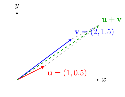
Geometric interpretation: Vector addition in $\mathbb{R}^2$ corresponds to the parallelogram law.
Subspaces
A subspace of a vector space \( V \) is a nonempty subset \( W \subseteq V \) that itself satisfies the conditions of a vector space. That is, \( W \) is closed under linear combinations:
If \( \mathbf{x}, \mathbf{y} \in W \), then \( \mathbf{x} + \mathbf{y} \in W \).
If \( c \in \mathbb{R} \) and \( \mathbf{x} \in W \), then \( c\mathbf{x} \in W \).
Thus, a subspace is a subset that is closed under vector addition and scalar multiplication. Because these operations already satisfy the eight vector space axioms in \( V \), they automatically hold in any subspace \( W \).
Note: Every subspace must contain the zero vector, since if \( \mathbf{x} \in W \), then \( 0\mathbf{x} = \mathbf{0} \in W \).
The possible subspaces of \( \mathbb{R}^3 \) include:
The zero subspace \( \{\mathbf{0}\} \)
Any line through the origin
Any plane through the origin
The entire space \( \mathbb{R}^3 \)
The smallest subspace is \( \{\mathbf{0}\} \), containing only the origin. The largest subspace is the whole space \( \mathbb{R}^3 \) itself.
Case 1: Consider all vectors in \( \mathbb{R}^2 \) with nonnegative components: \[ W = \{(x,y) \mid x \geq 0, \, y \geq 0\} \] This set is the first quadrant. It contains the zero vector and is closed under addition, but not under scalar multiplication. If we multiply \( (1,1) \) by \( -1 \), we get \( (-1,-1) \), which lies outside the first quadrant. Hence, \( W \) is not a subspace.
Case 2: If we include both the first and third quadrants, multiplication by negative scalars is allowed, but addition can move vectors out of these quadrants. Thus, even this enlarged set is not a subspace.
The smallest subspace containing the first quadrant is the entire \( \mathbb{R}^2 \).
Let \( V \) be the vector space of all \( 3 \times 3 \) matrices. Then the following are subspaces of \( V \):
The set of all lower triangular matrices
The set of all symmetric matrices
Both sets are closed under matrix addition and scalar multiplication, and contain the zero matrix.
For a matrix \( A \in \mathbb{R}^{m \times n} \), the column space of \( A \), denoted \( C(A) \), is the set of all linear combinations of the columns of \( A \): \[ C(A) = \{ A\mathbf{x} \mid \mathbf{x} \in \mathbb{R}^n \} \] It is a subspace of \( \mathbb{R}^m \).
The system \( A\mathbf{x} = \mathbf{b} \) is solvable if and only if \( \mathbf{b} \in C(A) \). That is, \( \mathbf{b} \) can be expressed as a linear combination of the columns of \( A \).
Consider \[ A = \begin{bmatrix} 1 & 0 \\ 5 & 4 \\ 2 & 4 \end{bmatrix}, \quad \mathbf{x} = \begin{bmatrix} u \\ v \end{bmatrix}, \quad \mathbf{b} = \begin{bmatrix} b_1 \\ b_2 \\ b_3 \end{bmatrix} \] Then \( A\mathbf{x} = \mathbf{b} \) means \[ u \begin{bmatrix} 1 \\ 5 \\ 2 \end{bmatrix} + v \begin{bmatrix} 0 \\ 4 \\ 4 \end{bmatrix} = \begin{bmatrix} b_1 \\ b_2 \\ b_3 \end{bmatrix}. \] All attainable right-hand sides \( \mathbf{b} \) lie in the plane spanned by the two column vectors of \( A \). This plane is the column space \( C(A) \subseteq \mathbb{R}^3 \).
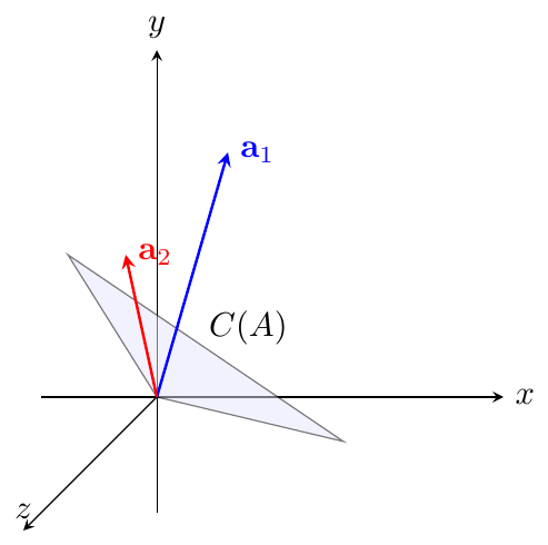
Figure: Column space \( C(A) \) is a plane through the origin in \( \mathbb{R}^3 \).
The nullspace of a matrix \( A \), denoted \( N(A) \), is the set of all vectors \( \mathbf{x} \in \mathbb{R}^n \) such that \[ A\mathbf{x} = \mathbf{0}. \] It is a subspace of \( \mathbb{R}^n \).
Properties:
If \( A\mathbf{x} = \mathbf{0} \) and \( A\mathbf{x}' = \mathbf{0} \), then \( A(\mathbf{x} + \mathbf{x}') = \mathbf{0} \).
If \( A\mathbf{x} = \mathbf{0} \), then \( A(c\mathbf{x}) = \mathbf{0} \) for any scalar \( c \).
Note: Only homogeneous systems (\( \mathbf{b} = 0 \)) form subspaces.
For \[ A = \begin{bmatrix} 1 & 0 \\ 5 & 4 \\ 2 & 4 \end{bmatrix}, \quad A\mathbf{x} = \mathbf{0} \Rightarrow \begin{cases} u = 0 \\ 5u + 4v = 0 \\ 2u + 4v = 0 \end{cases} \Rightarrow u = v = 0. \] Hence, \( N(A) = \{(0,0)\} \). The columns are linearly independent.
Now let \[ B = \begin{bmatrix} 1 & 0 & 1 \\ 5 & 4 & 9 \\ 2 & 4 & 6 \end{bmatrix}. \] Then \[ B \begin{bmatrix} c \\ c \\ -c \end{bmatrix} = \begin{bmatrix} 0 \\ 0 \\ 0 \end{bmatrix}. \] Thus, \( N(B) = \{ c(1,1,-1) \mid c \in \mathbb{R} \} \), which is a line through the origin — a one-dimensional subspace.
The column space \( C(A) \subseteq \mathbb{R}^m \) contains all attainable right-hand sides \( \mathbf{b} \) for \( A\mathbf{x} = \mathbf{b} \).
The nullspace \( N(A) \subseteq \mathbb{R}^n \) contains all solutions \( \mathbf{x} \) to \( A\mathbf{x} = 0 \).
Both are subspaces; they play a fundamental role in understanding linear systems.
Linear Independence, Basis, and Dimension
Linear Independence: A set of vectors $\{v_1, v_2, \dots, v_k\}$ is linearly independent if the equation \[ c_1 v_1 + c_2 v_2 + \dots + c_k v_k = 0 \] has only the trivial solution $c_1 = c_2 = \dots = c_k = 0$.
If there exists a nontrivial solution (some $c_i \neq 0$), the vectors are linearly dependent.
Let $v_1 = \begin{bmatrix}1\\1\\0\end{bmatrix}, v_2 = \begin{bmatrix}0\\1\\1\end{bmatrix}, v_3 = \begin{bmatrix}1\\2\\1\end{bmatrix}$ in $\mathbb{R}^3$.
Check $c_1 v_1 + c_2 v_2 + c_3 v_3 = 0$: \[ c_1 \begin{bmatrix}1\\1\\0\end{bmatrix} + c_2 \begin{bmatrix}0\\1\\1\end{bmatrix} + c_3 \begin{bmatrix}1\\2\\1\end{bmatrix} = \begin{bmatrix}0\\0\\0\end{bmatrix} \]
Solving gives $c_1 = c_2 = c_3 = 0$.
Hence, $\{v_1, v_2, v_3\}$ are linearly independent.
Let $v_1 = \begin{bmatrix}1\\2\end{bmatrix}, v_2 = \begin{bmatrix}2\\4\end{bmatrix}$ in $\mathbb{R}^2$.
Check $c_1 v_1 + c_2 v_2 = 0$: \[ c_1 \begin{bmatrix}1\\2\end{bmatrix} + c_2 \begin{bmatrix}2\\4\end{bmatrix} = \begin{bmatrix}0\\0\end{bmatrix} \]
A nontrivial solution exists: $c_1 = 2, c_2 = -1$.
Hence, $v_1$ and $v_2$ are linearly dependent.
Spanning a Subspace: A set of vectors $\{w_1, \dots, w_\ell\}$ spans a subspace $V$ if every vector $v \in V$ can be written as \[ v = c_1 w_1 + c_2 w_2 + \dots + c_\ell w_\ell \] for some scalars $c_1, \dots, c_\ell$.
In $\mathbb{R}^3$, vectors $w_1 = (1,0,0)$, $w_2 = (0,1,0)$, $w_3 = (1,1,0)$ span the $x$-$y$ plane.
Even $w_1$ and $w_2$ alone span the plane. $w_1$ and $w_3$ only span a line.
Let $A = \begin{bmatrix}1 & 2\\0 & 1\\1 & 1\end{bmatrix}$. The columns of $A$ span a subspace of $\mathbb{R}^3$. Any vector $v$ in this subspace can be written as $v = c_1 \begin{bmatrix}1\\0\\1\end{bmatrix} + c_2 \begin{bmatrix}2\\1\\1\end{bmatrix}$.
Basis of a Vector Space: A basis of a vector space $V$ is a set of vectors that
are linearly independent, and
span $V$.
Every vector in $V$ can then be expressed uniquely as a linear combination of basis vectors.
In $\mathbb{R}^2$, vectors $v_1 = (1,2)$, $v_2 = (2,3)$ are linearly independent and span $\mathbb{R}^2$.
Hence, $\{v_1, v_2\}$ is a basis of $\mathbb{R}^2$.
For the matrix $A = \begin{bmatrix}1 & 3 & 1\\0 & 1 & 2\\0 & 0 & 1\end{bmatrix}$, pivot columns are 1, 2, 3. These columns form a basis of the column space of $A$.
Dimension of a Vector Space: The number of vectors in any basis of a vector space $V$ is called the dimension of $V$, denoted $\dim(V)$.
All bases of $V$ have the same number of vectors.
- $R^3$ has dimension 3. Standard basis: $e_1=(1,0,0)$, $e_2=(0,1,0)$, $e_3=(0,0,1)$. - $x$-$y$ plane in $\mathbb{R}^3$ has dimension 2.
Matrix $A = \begin{bmatrix}1 & 3 & 3 & 2 \\ 0 & 0 & 3 & 1 \\ 0 & 0 & 0 & 0\end{bmatrix}$ has pivot columns 1 and 3. Dimension of the column space = 2.
Rank and Linear Independence:
The rank of a matrix $A$ = number of independent rows or columns.
Rank = dimension of column space = dimension of row space.
If $n > m$ in an $m \times n$ matrix, the $n$ columns are dependent.
Consider $A = \begin{bmatrix}1 & 2 & 3\\2 & 4 & 6\end{bmatrix}$. - $m=2, n=3$, so $n>m$. - Rank = 1 (only first column is independent). - All 3 columns are linearly dependent.
Let $U = \begin{bmatrix}1 & 2 & 0\\0 & 1 & 1\\0 & 0 & 0\end{bmatrix}$. - Pivot columns: 1 and 2. - Basis for column space: columns 1 and 2. - Dimension = rank = 2.
Key Theorems:
Any set of more than $n$ vectors in $\mathbb{R}^n$ is linearly dependent.
A linearly independent set can be extended to a basis.
A spanning set can be reduced to a basis.
All bases of a vector space have the same number of vectors.
Applications of Vector Spaces
Vector spaces provide a framework to understand solutions of linear systems $Ax = b$.
- The column space $C(A)$ determines whether $b$ lies in the span of the columns. - The nullspace $N(A)$ gives all solutions of the homogeneous system $Ax = 0$. - The rank of $A$ tells the number of independent equations. - A basis of $C(A)$ allows expressing any solution as a linear combination of independent columns.
Vector spaces represent points, directions, and transformations in 2D/3D graphics.
- Any point or vector can be expressed as a combination of basis vectors. - Linear transformations like rotations, scaling, and projections are matrix operations on vector spaces.
Signals are represented as vectors in function spaces or discrete vector spaces.
- Orthogonal bases, such as Fourier or wavelet bases, allow decomposition into independent components. - The dimension of the vector space corresponds to the number of independent signal components.
Feature vectors in machine learning exist in high-dimensional vector spaces.
- Linear independence ensures that features are non-redundant. - Basis vectors can be used for dimensionality reduction, e.g., in Principal Component Analysis (PCA). - Rank of the data matrix reveals the intrinsic dimensionality of the dataset.
Vector spaces describe physical quantities such as forces, velocities, and fields.
- Basis vectors often correspond to orthogonal coordinate axes. - Linear independence ensures that combinations of forces or fields can be uniquely represented. - The dimension of the space corresponds to the number of independent physical directions.
State-space models use vectors for system states and inputs.
- Linear independence of state vectors is crucial for controllability and observability. - Dimension of the state-space corresponds to the number of independent states of the system.