The Data
Data Objects and Attribute Types
A data object represents an entity in a dataset.
Also called: samples, instances, data points, tuples
Each row in a database table $\rightarrow$ one data object
Described by a set of attributes
An attribute is a data field representing a characteristic of a data object.
Also called: feature, variable, dimension, field
Example:
Age,Name,Salary,Zip Code
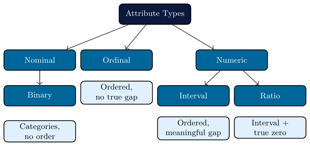
Nominal Attributes
A nominal attribute takes values that are names or labels for categories.
No ordering between values — cannot say one is greater or lesser
No arithmetic meaningful — mean, sum have no sense
Only valid operations: equality (=) and inequality ($\neq$)
Mode is the only meaningful central tendency measure
Values act as labels only — even if coded as numbers (e.g.\ 1=red, 2=blue), arithmetic is meaningless
Can be multi-valued: one object may belong to multiple categories
Useful statistics: frequency count, mode, contingency tables
Attribute: HairColor Domain: {Black, Brown, Blonde, Red, Gray}
Person A $\rightarrow$ Black Person B $\rightarrow$ Blonde Person C $\rightarrow$ Red
We can say: A $\neq$ B
We cannot say: Black $>$ Blonde, or Average(Black, Red) = ?
Most frequent value (mode) $\rightarrow$ valid summary statistic
Attribute: Occupation Domain: {Doctor, Engineer, Teacher, Lawyer, Artist}
Encoded internally as: Doctor=1, Engineer=2, Teacher=3, Lawyer=4, Artist=5
Even though stored as numbers, $1 + 2 = 3$ (Doctor + Engineer = Teacher?)
Only meaningful question: “How many people are Engineers?” $\rightarrow$ frequency count
Ordering like Engineer $>$ Doctor is completely invalid
Attribute: PinCode Example values: {110001, 560001, 400001}
Looks numeric — but arithmetic is meaningless
$560001 - 110001 = 450000$ has no geographic meaning
Used only to identify a region (label), not to measure anything
Correct use: grouping, frequency, equality checks only
Binary Attributes
A binary attribute is a special case of nominal with exactly two possible states: 0 and 1 (or True/False, Yes/No).
Symmetric binary — both outcomes carry equal weight/importance
Asymmetric binary — one outcome is more significant (usually coded as 1)
Symmetric: Neither state is more important
Example:Gender— Male and Female are equally weightedAsymmetric: State 1 (positive) is rare and more important
Example:Disease Diagnosis— Positive is rare, but criticalFor similarity measures, asymmetric binary attributes ignore 0-0 matches (both negative = uninformative)
Attribute: HIV_Test States: {Positive=1, Negative=0}
Most patients test Negative (0) — this is the common, uninformative state
A Positive (1) result is rare and highly significant
When comparing two patients, a 1-1 match (both positive) is very meaningful
A 0-0 match (both negative) is ignored in similarity computation — it adds no information
Jaccard coefficient used instead of simple matching coefficient
Attribute: Gender States: {Male=1, Female=0} (or vice versa)
Both states are equally important — no state is rarer or more critical
A 0-0 match (both Female) is just as meaningful as a 1-1 match (both Male)
Simple matching coefficient is appropriate for similarity
Recoding Male=0, Female=1 does not change the analysis
Attribute: Bought_Item States: {Yes=1, No=0}
In a large transaction database, most entries are 0 (item not bought)
A 1-1 co-occurrence (two customers both buying the same item) $\rightarrow$ meaningful pattern
0-0 co-occurrence (both did not buy) $\rightarrow$ uninformative, ignored
Used heavily in market basket analysis and association rule mining
Ordinal Attributes
An ordinal attribute has values with a meaningful rank order, but the magnitude of difference between successive values is unknown.
Valid operations: =, $\neq$, $<$, $>$, $\leq$, $\geq$
Cannot compute meaningful differences: $A - B$ has no fixed meaning
Central tendency: median and mode are valid; mean is not
If an ordinal attribute has $M$ states (ordered $1$ to $M$), values can be mapped to $[0,1]$: \[ z_i = \frac{r_i - 1}{M - 1}, \quad r_i \in \{1, 2, \ldots, M\} \] This allows ordinal data to be used in certain numeric computations (e.g., distance measures).
Attribute: Grade Order: F $<$ D $<$ C $<$ B $<$ A
Student X: B Student Y: A Student Z: C
We know: A $>$ B $>$ C
We cannot say: the gap between A and B equals the gap between B and C
Median grade of {B, A, C, B, D} = B (after sorting: D, C, B, B, A)
Mean of {B, A, C} = ? undefined and meaningless
Attribute: Satisfaction Order: Very Dissatisfied $<$ Dissatisfied $<$ Neutral $<$ Satisfied $<$ Very Satisfied
$M = 5$ states, mapped: Very Dissatisfied=1, …, Very Satisfied=5
Normalized: $z = \{0,\ 0.25,\ 0.5,\ 0.75,\ 1.0\}$
“Satisfied” is better than “Neutral” — but by how much? Unknown
Report median satisfaction, not average — averaging ordinal labels is statistically incorrect
Attribute: Rank Order: Private $<$ Corporal $<$ Sergeant $<$ Lieutenant $<$ Captain
Clear ordering of authority and responsibility
Sergeant is higher than Corporal
(Captain $-$ Lieutenant) = (Sergeant $-$ Corporal)? No such claim valid
Useful in sorting, ranking comparisons, and ordinal regression models
Numeric Attributes
A numeric attribute is quantitative — represented by measurable numbers with meaningful arithmetic.
Two subtypes:
Interval-scaled — ordered, meaningful differences, no true zero
Ratio-scaled — interval + true zero, all arithmetic valid
Interval-Scaled Attributes
Measured on a scale with equal-sized units
Differences are meaningful; ratios are not
No absolute zero — zero is just another point on the scale
Valid operations: $+$, $-$ Invalid: $\times$, $\div$ for ratio comparisons
Attribute: Temperature_C
$30^\circ C - 20^\circ C = 10^\circ C$ difference is meaningful
$40^\circ C$ is NOT twice as hot as $20^\circ C$
Proof: $40^\circ C = 104^\circ F$, $20^\circ C = 68^\circ F$, $104/68 \neq 2$ — ratio changes with scale
$0^\circ C$ does not mean absence of heat — water still has thermal energy
Attribute: Year
$2024 - 2020 = 4$ years difference
Year 2024 is not “twice” as recent as Year 1012
Year 0 is an arbitrary reference, not the start of time
Differences (durations) are meaningful; ratios of years are not
Ratio-Scaled Attributes
Has all properties of interval plus a true zero
Zero means complete absence of the quantity
All arithmetic valid: $+$, $-$, $\times$, $\div$
Can make statements like “X is twice as much as Y”
Attribute: Weight_kg
Person A: 80 kg Person B: 40 kg
A is exactly twice as heavy as B $80/40 = 2$
0 kg = truly no weight
Difference: $80 - 40 = 40$ kg meaningful
Mean, variance, standard deviation all valid
Attribute: Annual_Salary
Salary of $0 = no income (true zero)
$80,000 is four times $20,000
Meaningful to compute: average salary, salary ratio, percentage increase
Transformations (log scale) commonly applied for skewed salary distributions
Attribute: Age_years
Age 0 = just born — true absence of elapsed life time
Person aged 60 is twice as old as person aged 30
Difference: $60 - 30 = 30$ years, fully meaningful
Mean age, age ratio — all statistically valid operations
Discrete versus Continuous Attributes
A discrete attribute has a finite or countably infinite set of values.
Values are distinct, separate — no value exists between two adjacent values
Often represented as integers
Nominal and ordinal attributes are always discrete
Some numeric attributes are also discrete (e.g., count data)
A continuous attribute can take any real value within a range.
Infinite possible values between any two points
Represented as floating-point numbers in practice
Measurements (height, weight, temperature) are typically continuous
In practice, precision of instrument limits the recorded values
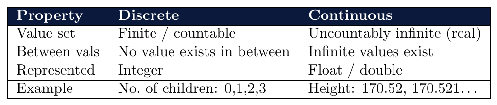
Attribute: Items_Purchased Domain: {0, 1, 2, 3, …}
A customer can buy 3 or 4 items — never 3.5 items
Set is countably infinite — no upper bound, but each value is a whole number
Represented as integer; bar charts and frequency tables are natural visualizations
Mean is technically computable but result (e.g., 2.7 items) must be interpreted carefully
Attribute: PinCode Example: {110001, 560001, 400001}
Finite set of valid pin codes across the country
No pin code exists between 110001 and 110002 — they are adjacent, distinct labels
Although stored as numbers, this is a nominal discrete attribute
Frequency analysis by pin code region is a valid operation
Attribute: Height_cm Example: 170.5, 171.2, 165.87
Between 170 cm and 171 cm, infinitely many real values exist: 170.1, 170.11, 170.111…
Measured by instrument — precision limited (e.g., 0.1 cm), but the attribute itself is continuous
Histograms (not bar charts) are the appropriate visualization
All statistical operations valid: mean, variance, percentile, standard deviation
Attribute: Temperature_C
Can be 36.6, 36.61, 36.612… — infinite precision possible
Thermometer records to 1 decimal, but true value is continuous
In data preprocessing: often discretized into bins
e.g., $[<20^\circ C =$ Cold$]$, $[20$–$35^\circ C =$ Warm$]$, $[>35^\circ C =$ Hot$]$Discretization converts continuous $\rightarrow$ ordinal for certain algorithms
Basic Statistical Descriptions of Data
Helps understand the distribution and spread of data
Identifies outliers, noise, and skewness early
Guides preprocessing decisions: normalization, binning, transformation
Measuring the Central Tendency: Mean, Median, and Mode
A central tendency measure gives a single value that best represents an entire dataset.
Three primary measures:
Mean — arithmetic average
Median — middle value when sorted
Mode — most frequently occurring value
Mean
For $N$ values $x_1, x_2, \ldots, x_N$: \[ \bar{x} = \frac{1}{N} \sum_{i=1}^{N} x_i \]
Most common measure of central tendency
Sensitive to outliers — a single extreme value pulls the mean strongly
Valid only for interval and ratio attributes
When values have different importance (weights $w_i$): \[ \bar{x}_w = \frac{\sum_{i=1}^{N} w_i x_i}{\sum_{i=1}^{N} w_i} \] Used when some observations are more reliable or frequent than others.
Remove a fixed percentage of extreme values (top and bottom) before computing mean
Reduces effect of outliers
Example: 5% trimmed mean — discard lowest 5% and highest 5% of values
Scores of 7 students: {52, 60, 65, 70, 72, 80, 95}
\[
\bar{x} = \frac{52 + 60 + 65 + 70 + 72 + 80 + 95}{7} = \frac{494}{7} \approx 70.57
\]
If one student scored 200 (data error), mean becomes $\approx 99.14$ — heavily distorted
This shows mean's sensitivity to outliers
Three components with weights:
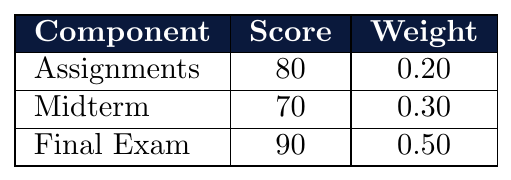
\[ \bar{x}_w = \frac{(80 \times 0.20) + (70 \times 0.30) + (90 \times 0.50)}{0.20 + 0.30 + 0.50} = \frac{16 + 21 + 45}{1} = 82 \] Simple mean would give $\frac{80+70+90}{3} = 80$ — ignoring the higher importance of the final exam.
Median
The median is the middle value of a sorted dataset. \[ \text{Median} = \begin{cases} x_{\left(\frac{N+1}{2}\right)} & \text{if } N \text{ is odd} \\[6pt] \dfrac{x_{\left(\frac{N}{2}\right)} + x_{\left(\frac{N}{2}+1\right)}}{2} & \text{if } N \text{ is even} \end{cases} \]
Not affected by outliers — robust measure
Preferred over mean when data is skewed
Valid for ordinal, interval, and ratio attributes
When data is in frequency classes, median is estimated as:
\[
\text{Median} = L_1 + \left(\frac{\frac{N}{2} - \sum f_l}{f_{\text{median}}}\right) \times \text{width}
\]
where $L_1$ = lower boundary of median class, $\sum f_l$ = frequencies before median class,
$f_{\text{median}}$ = frequency of median class, width = class interval width.
Salaries (in thousands): {30, 45, 50, 60, 72, 85, 120} $N = 7$
Sorted (already sorted above)
Middle position: $\frac{7+1}{2} = 4$th value
Median $= 60$
Note: even if the outlier 120 becomes 5000, median remains 60
House prices (lakhs): {25, 40, 55, 70, 90, 130} $N = 6$
Positions $\frac{6}{2} = 3$rd and $4$th values: 55 and 70
Median $= \dfrac{55 + 70}{2} = 62.5$ lakhs
Mean $= \dfrac{25+40+55+70+90+130}{6} = 68.3$ lakhs — pulled up by 130
Median better represents the “typical” house price here
Mode
The mode is the value that occurs most frequently in a dataset.
A dataset can be unimodal (one mode), bimodal (two modes), or multimodal
Valid for all attribute types including nominal
For continuous data: mode is estimated from the most frequent class interval
For moderately skewed unimodal distributions: \[ \text{Mean} - \text{Mode} \approx 3 \times (\text{Mean} - \text{Median}) \]
Symmetric distribution: Mean $=$ Median $=$ Mode
Positively skewed (right): Mode $<$ Median $<$ Mean
Negatively skewed (left): Mean $<$ Median $<$ Mode
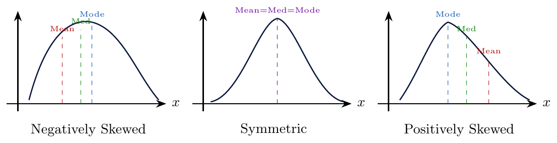
Sizes sold in a day: {6, 7, 7, 8, 8, 8, 9, 9, 10}
Size 8 appears 3 times — most frequent
Mode $= 8$ (unimodal)
A store manager stocks more of size 8 based on mode — not mean or median
Mode is the only valid central tendency for nominal data
Ages: {18, 19, 20, 20, 21, 35, 36, 36, 37, 38}
Mode $= 20$ and $36$ — bimodal distribution
Reveals two distinct groups: college students and working professionals
Mean $\approx 27.9$ — falls in a gap between both groups, misrepresenting either group
Bimodal patterns suggest the data may need to be split into subgroups
Measuring the Dispersion of Data
Dispersion measures how spread out the data values are around the central tendency.
Low dispersion $\rightarrow$ values clustered tightly around the mean
High dispersion $\rightarrow$ values scattered widely
Key measures: Range, Quartiles, IQR, Variance, Standard Deviation
Range
\[ \text{Range} = x_{\max} - x_{\min} \]
Simplest measure of spread
Extremely sensitive to outliers — one bad value distorts it completely
Gives no information about how values are distributed within the range
Rainfall (mm): {10, 25, 40, 55, 70, 120}
\[
\text{Range} = 120 - 10 = 110 \text{ mm}
\]
If 120 is an outlier (measurement error), range is completely misleading
IQR and standard deviation give a more reliable picture
Quartiles and IQR
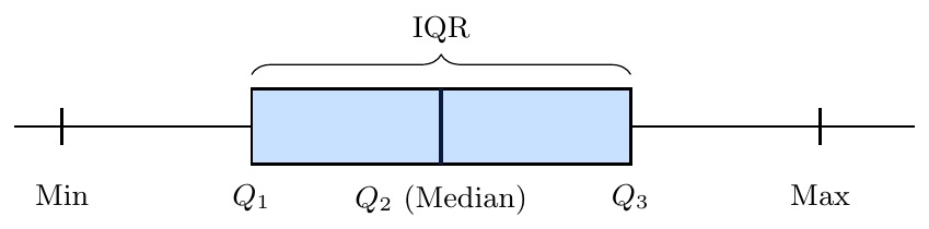
Quartiles divide a sorted dataset into four equal parts:
$Q_1$ (25th percentile) — 25% of data lies below this value
$Q_2$ (50th percentile) — the median
$Q_3$ (75th percentile) — 75% of data lies below this value
\[ \text{IQR} = Q_3 - Q_1 \]
A value is considered an outlier if it falls outside the fences: \[ \text{Lower fence} = Q_1 - 1.5 \times \text{IQR} \qquad \text{Upper fence} = Q_3 + 1.5 \times \text{IQR} \] Any value beyond these fences is flagged as a potential outlier.
Scores (sorted): {42, 55, 60, 65, 70, 75, 80, 88, 95} $N=9$
$Q_2$ = 5th value $= 70$
$Q_1$ = median of lower half {42, 55, 60, 65} $= \dfrac{60+55}{2} = 57.5$
$Q_3$ = median of upper half {75, 80, 88, 95} $= \dfrac{80+88}{2} = 84$
$\text{IQR} = 84 - 57.5 = 26.5$
Lower fence $= 57.5 - 1.5(26.5) = 17.75$ Upper fence $= 84 + 1.5(26.5) = 123.75$
All values within fences — no outliers in this dataset
Salaries (thousands): {30, 35, 38, 40, 42, 45, 48, 50, 200}
$Q_1 = 38$, $Q_3 = 48$, $\text{IQR} = 10$
Upper fence $= 48 + 1.5 \times 10 = 63$
Salary of 200 exceeds 63 — flagged as outlier
Without IQR, range $= 170$ makes the spread look enormous; IQR $= 10$ reveals true spread
Variance and Standard Deviation
Variance measures the average squared deviation from the mean: \[ \sigma^2 = \frac{1}{N} \sum_{i=1}^{N} (x_i - \bar{x})^2 \] Standard Deviation is the square root of variance — in the same units as the data: \[ \sigma = \sqrt{\frac{1}{N} \sum_{i=1}^{N} (x_i - \bar{x})^2} \]
Low $\sigma$ $\rightarrow$ values clustered near mean
High $\sigma$ $\rightarrow$ values spread widely
Sensitive to outliers — squaring amplifies extreme deviations
Population variance: divide by $N$
Sample variance: divide by $N-1$ (Bessel's correction — avoids underestimation) \[ s^2 = \frac{1}{N-1} \sum_{i=1}^{N} (x_i - \bar{x})^2 \]
In data mining, population formula is commonly used when entire dataset is available
Temperatures ($^\circ$C): {20, 22, 24, 26, 28} $\bar{x} = 24$
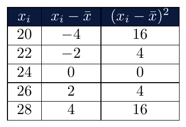
\[ \sigma^2 = \frac{16+4+0+4+16}{5} = \frac{40}{5} = 8 \qquad \sigma = \sqrt{8} \approx 2.83^\circ C \] Temperatures deviate on average by $2.83^\circ C$ from the mean of $24^\circ C$.
Batsman A scores: {45, 48, 50, 52, 55} $\bar{x} = 50$
Batsman B scores: {10, 30, 50, 70, 90} $\bar{x} = 50$
Both have the same mean: 50
$\sigma_A = \sqrt{\frac{(-5)^2+(-2)^2+0^2+2^2+5^2}{5}} = \sqrt{11.6} \approx 3.4$
$\sigma_B = \sqrt{\frac{(-40)^2+(-20)^2+0^2+20^2+40^2}{5}} = \sqrt{1200} \approx 34.6$
Batsman A is consistent (low $\sigma$); Batsman B is unpredictable (high $\sigma$)
Mean alone is completely insufficient to compare performance