Algorithm Analysis
Introduction
A data structure is a way to store data in a computer so that we can use it easily. Just like we keep clothes in a cupboard with shelves, so that we find them fast, a data structure keeps data in an organised way. Different data structures store data in different ways. We pick the right one based on what work we want to do with the data.
Think of a train. Each bogie is connected to the next bogie in a line. This is like a Linked List data structure, where one item points to the next item.
Suppose we want to check if a webpage URL is already visited or not, very fast, again and again. Which data structure suits best, a List or a Hash Table? A Hash Table suits best here, because checking an item in a Hash Table takes less time on average than checking in a List.
An algorithm is a step by step method to solve a problem. It is like a recipe to cook food. The recipe tells what to do first, what to do next, and what to do last. An algorithm takes some input, does some steps, and gives an output. A good algorithm should be clear, correct, and should finish in finite steps.
To make tea, we follow steps. Boil water, add tea powder, add milk, add sugar, boil again, and pour in a cup. This is an algorithm, because it has clear steps in a fixed order.
Given an array $A = [4, 9, 2, 7, 1]$, an algorithm to find the maximum number will compare each element one by one with a variable holding the current maximum, and update it when a bigger number is found. At the end, the variable holds the maximum value, which is $9$.
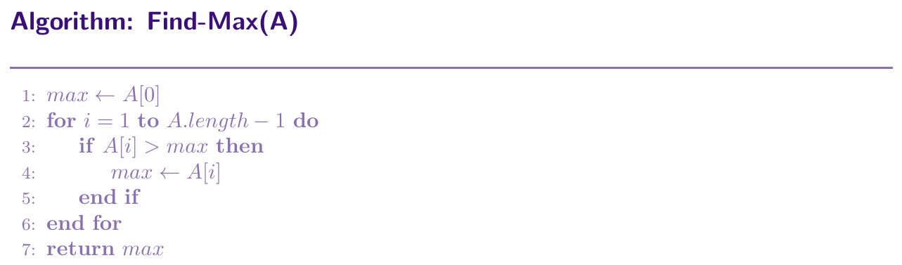
Pseudocode is a simple way to write the steps of an algorithm using plain words and simple structure, similar to a programming language but not exact. It is not a real programming language, so we cannot run it on a computer. It helps us to plan the logic first, before writing real code. We write it using simple words like if, for, while, so anyone can understand it easily.
Find-Max(A)
max = A[0]
for i = 1 to length(A) - 1
if A[i] $>$ max
max = A[i]
return max
Code is the actual set of instructions written in a programming language, which a computer can run directly. We take the logic from pseudocode and convert it into Python code, following Python rules like indentation and syntax. Once written, this code can be run on a computer to get the real output.
def find_max(arr):
    max_val = arr[0]
    for i in range(1, len(arr)):
        if arr[i] > max_val:
            max_val = arr[i]
    return max_val
Core Algorithmic Paradigms
Brute force means we check every possible option one by one, until we find the correct answer. We do not use any trick or shortcut. It is simple to think and write, but it can take a lot of time when the number of options is large.
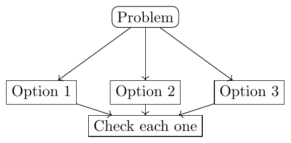
Suppose we want to find two numbers in a list that add up to a target value. Brute force will pick every pair of numbers, one pair at a time, and check if their sum matches the target. It keeps doing this for all possible pairs.
This method breaks a big problem into smaller parts, called subproblems. These subproblems are independent of each other, which means one subproblem does not depend on another. We solve each small part separately, and then we combine all the small answers to get the final answer.
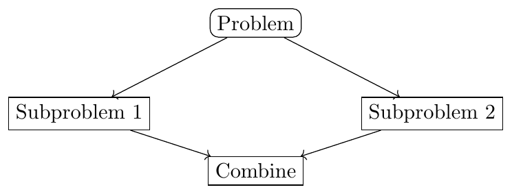
Suppose we want to sort a big list of numbers. Divide and conquer will split the list into two halves, sort each half on its own, and then join the two sorted halves into one sorted list.
This method reduces the problem to one smaller problem of the same type, not many. We solve that one smaller problem, and then we use its answer to build the answer for the original problem.
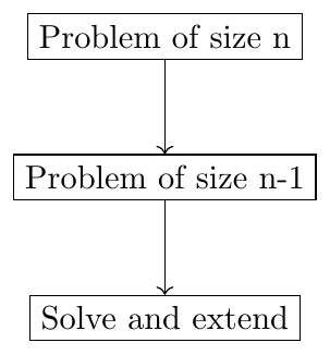
Suppose we want to find the maximum number in a list. Decrease and conquer will find the maximum in the list without the last element, which is a smaller problem, and then compare that result with the last element to get the final maximum.
This method changes the problem into a different, simpler form, which is easier to solve. After solving the new simpler form, we use that result for our original problem.
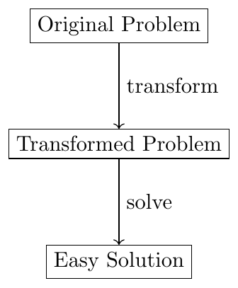
Suppose we want to check if a list has any duplicate numbers. Transform and conquer will first sort the list, which is a transformation, and then simply check neighbouring elements, which becomes a much easier check.
This method picks the best option available right now, at every step, without thinking about the future steps. It hopes that picking the best choice every time will give the best overall answer at the end.
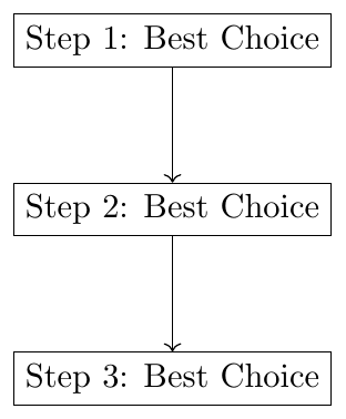
Suppose we want to give change to a customer using minimum number of coins. Greedy method will always pick the largest coin value possible at each step, until the full change amount is given.
This method also breaks a problem into smaller subproblems, like divide and conquer. But here, the same subproblem can come again and again, so we store the answer of each subproblem once, and reuse it later instead of solving it again.
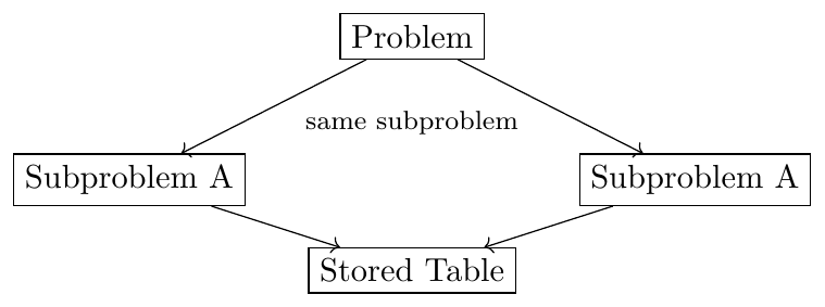
Suppose we want to find the number of ways to climb a staircase, taking one or two steps at a time. Dynamic programming will store the number of ways for each smaller staircase height, and reuse those stored values to build the answer for the full staircase.
This method builds a solution step by step. At each step, if we find that the current path breaks a rule of the problem, we go back to the previous step and try a different option. This way, we avoid wrong paths early.
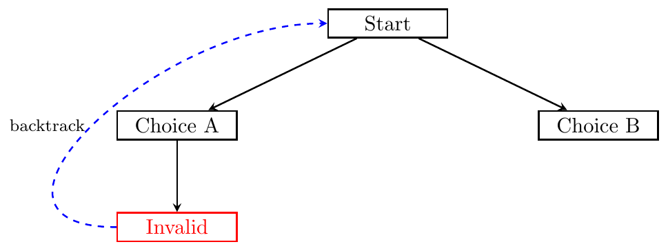
Suppose we want to place numbers in a sudoku grid. Backtracking will place a number in a cell, and if it breaks a sudoku rule, it removes that number and tries the next possible number in that cell.
This method is used for optimization problems, where we want the best possible answer, like minimum cost or maximum profit. It builds a tree of choices, and at each branch, it calculates a bound, which tells if that branch can possibly give a better answer or not. If a branch cannot give a better answer, we cut it off and do not explore it further.
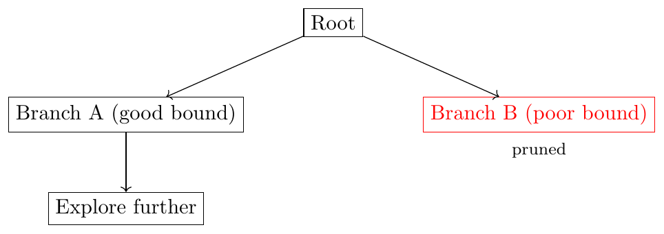
Suppose a delivery person wants the shortest route to visit many cities. Branch and bound will build partial routes, calculate a lower bound cost for each partial route, and skip any partial route whose bound is already worse than the best route found so far.
Analysis Framework
Time and Space Efficiency
We check how good an algorithm is using two things, time and space. Time efficiency means how long the algorithm takes to run. Space efficiency means how much extra memory the algorithm needs, apart from the input and output.
Think of cooking food. Time efficiency is like how many minutes the cooking takes. Space efficiency is like how many extra vessels and counter space we need while cooking, apart from the raw ingredients and the final dish.
Nowadays, computers have a lot of memory. So memory is not a big problem most of the time. But running time is still important, because we want answers fast. So, in most cases, we focus more on time efficiency than space efficiency.
Input Size and Efficiency Analysis
The work done by an algorithm depends on how big the input is. A bigger input usually means more work. So, we write the running time as a function of a number $n$, which represents the size of the input.
Sweeping a small room takes less time. Sweeping a big hall takes more time. Here, the size of the room is like input size $n$, and the sweeping time grows as the room size grows.
For most problems, we pick the input size directly from the data we are given, like the number of elements in a list, the number of rows in a table, or the number of terms in an expression. Small differences in counting do not change our final conclusion about efficiency.
Suppose we want to check if a student ID is present in a record file. The algorithm reads each record one by one, compares the ID, and stops when found or when the file ends. If the file has $n$ records, the algorithm may check up to $n$ records in the worst case. If the file size doubles, the work also doubles. So here, input size is the number of records.
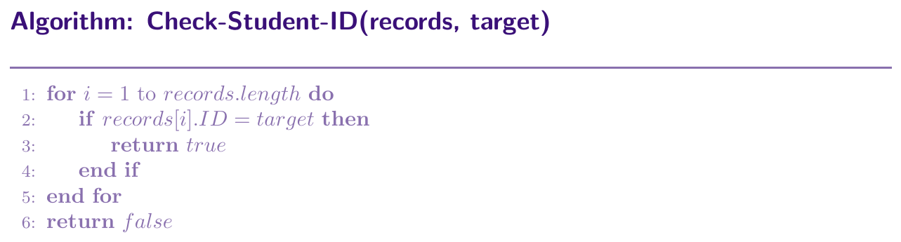
Some problems can have more than one way to measure input size. The algorithm itself does not change, but the way we write its growth function changes, depending on which size measure we choose.
For a matrix, we can measure size as the number of rows, or as the total number of elements (rows times columns). Both are valid, but the growth function looks different depending on which one we use.
We should choose the size measure based on what unit the algorithm actually works on. If the algorithm works on characters, we count characters. If it works on records or rows, we count those instead.
An algorithm that checks spelling works on each character of a word, so its input size is the number of characters. An algorithm that counts how many words are in a sentence works on each word, so its input size is the number of words.
Measuring Running Time of Algorithms
We should not measure an algorithm using seconds or milliseconds. This is because clock time depends on many outside things, like processor speed, programming language used, coding style, and how busy the system is at that moment. These things are not part of the algorithm. So, clock time does not give a fair measure of how good an algorithm is.
If two cooks use the same recipe, but one has a fast gas stove and the other has a slow stove, their cooking time will differ. But the recipe, that is the method, is the same for both. So, we should judge the recipe by its steps, not by the stove used.
Instead of checking how many seconds an algorithm takes, we count how many times an important operation runs. This count does not depend on the computer used. We do not count every single operation, we only count the operation that takes the most work.
The basic operation is the one operation that takes the most time in an algorithm. It is usually present inside the innermost loop, and it is the heaviest step in the algorithm. For example, comparing two elements in sorting, comparing two records in searching, or doing a division in a number based algorithm.
Suppose we want to check if a registration number is present in a list of employee records. The algorithm compares the target number with each record one by one, and stops when it matches or the list ends. Here, the basic operation is the comparison between two numbers. If the list has $n$ records, the algorithm does at most $n$ comparisons.
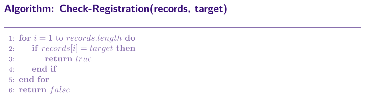
We can write the number of basic operations needed for input size $n$ as $C(n)$. We also have $c_{op}$, which is the time taken for one basic operation. Using these, we can estimate the running time as \[ T(n) \approx c_{op} \cdot C(n) \] This gives us a rough idea of running time, without depending on the actual machine timing.
If checking one record takes $c_{op}$ time, and we have $n$ records, then in the worst case, the total time is approximately $c_{op} \cdot n$. If $n$ becomes double, the total time also becomes roughly double.
When we study efficiency, we ignore constant multipliers. This is because these constants depend on the hardware and the way the program is written. Also, when input size becomes very large, these constants do not matter much, because the growth pattern of $C(n)$ matters more than the fixed constant.
If an algorithm takes $5n$ steps and another takes $2n$ steps, both grow in the same straight line pattern as $n$ increases. So, we say both algorithms have the same growth pattern, and we ignore the constants $5$ and $2$ while comparing their efficiency.
Order of Growth
When we compare algorithms, the difference does not show much when the input is small, because even a slow algorithm finishes fast for small input. The real difference is seen when the input size becomes very large. So, we study how the running time grows as the input size grows.
If an algorithm's operation count grows slowly as input size increases, the algorithm stays usable even for large problems. But if the operation count grows very fast, the algorithm becomes useless for large input. Because of this, we classify algorithms by their order of growth, which means how fast their cost increases with input size.
For a short distance, walking and running may take almost the same time. But for a very long road, running clearly takes much less time than walking. In the same way, for small input, slow and fast algorithms look similar, but for large input, the difference becomes clear.
We compare algorithms based on how the number of basic operations grows with input size $n$, not based on actual running time for small inputs. Different growth rates behave very differently:
Logarithmic growth ($\log n$) increases very slowly.
Linear growth ($n$) increases in direct proportion to input size.
Polynomial growth ($n^2$, $n^3$) increases fast.
Exponential ($2^n$) and factorial ($n!$) growth increase extremely fast, becoming unusable very quickly.
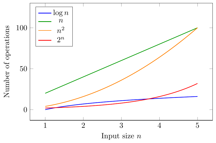
When we write $\log n$, the base of the log does not matter in efficiency analysis. This is because changing the base only changes the value by a constant factor, as shown below \[ \log_a n = \frac{\log_b n}{\log_b a} \] Since we ignore constant factors in this kind of analysis, we simply write $\log n$ without mentioning the base.
Algorithms with exponential growth ($2^n$) or factorial growth ($n!$) are practical only for very small input sizes. As $n$ increases even a little, their running time increases extremely fast, making them unusable for large input.
Suppose an algorithm needs $f(n) = n^2$ operations. If input size becomes double, from $n$ to $2n$, then \[ f(2n) = (2n)^2 = 4n^2 \] So the work becomes four times more.
Now suppose another algorithm needs $g(n) = n$ operations. If input size becomes double, then \[ g(2n) = 2n \] So the work becomes only double.
This shows that even if both algorithms look similar for small input, the algorithm with $n^2$ becomes much costlier than the algorithm with $n$, as input size grows large.
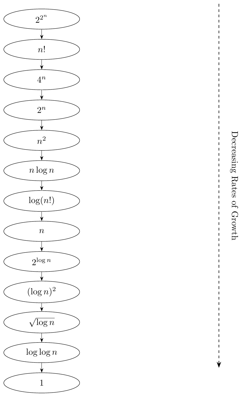
Arrange the following functions in increasing order of growth: \[ n, \log n, n^2, 1 \] Order: $1 < \log n < n < n^2$
Arrange the following functions in increasing order of growth: \[ n!, 2^n, n^3, n \log n \] Order: $n \log n < n^3 < 2^n < n!$
Arrange the following functions in increasing order of growth: \[ \sqrt{n}, n, \log n, n^2 \log n \] Order: $\log n < \sqrt{n} < n < n^2 \log n$
Arrange the following functions in increasing order of growth: \[ 2^n, n^{10}, 10^n, \log_2 n \] Order: $\log_2 n < n^{10} < 2^n < 10^n$
Arrange the following functions in increasing order of growth: \[ n \log n, n^2, n, 2^{\log n} \] Hint: simplify $2^{\log n}$ first using log identity, base 2.
Order: $n = 2^{\log n} < n \log n < n^2$
Asymptotic Notations
Asymptotic Efficiency of Algorithms
When input size becomes very large, small parts of the running time formula stop mattering. Constant numbers and small extra terms become tiny compared to the main growing part. So, we only look at the main part that grows with $n$. This way of studying growth is called asymptotic efficiency analysis.
If we buy 2 apples, paying 5 rupees extra for a bag does matter. But if we buy 1000 apples, that same 5 rupees extra does not matter much. In the same way, small constants in running time do not matter when input size is very large.
Asymptotic analysis tells us how well an algorithm scales, that means how it behaves as input grows bigger and bigger. It does not give us the exact running time in seconds. It only tells us the pattern of growth, which is the main thing we need while choosing an algorithm for large input.
A running time formula can have many terms, like $n^2 + 3n + 7$. As $n$ becomes very large, the term $n^2$ becomes much bigger than $3n$ and $7$. So, $3n$ and $7$ become useless in comparison. We only keep the dominant term, which is the term that grows the fastest, and we ignore the rest.
Mathematical view: Consider $f(n) = n^2 + 3n + 7$. We can divide every term by $n^2$ to see their relative size as $n$ grows: \[ \frac{f(n)}{n^2} = 1 + \frac{3}{n} + \frac{7}{n^2} \] As $n \to \infty$, the terms $\dfrac{3}{n}$ and $\dfrac{7}{n^2}$ become almost $0$. So, $f(n)$ behaves almost exactly like $n^2$ for large $n$. This is why we say $f(n)$ has order of growth $n^2$.
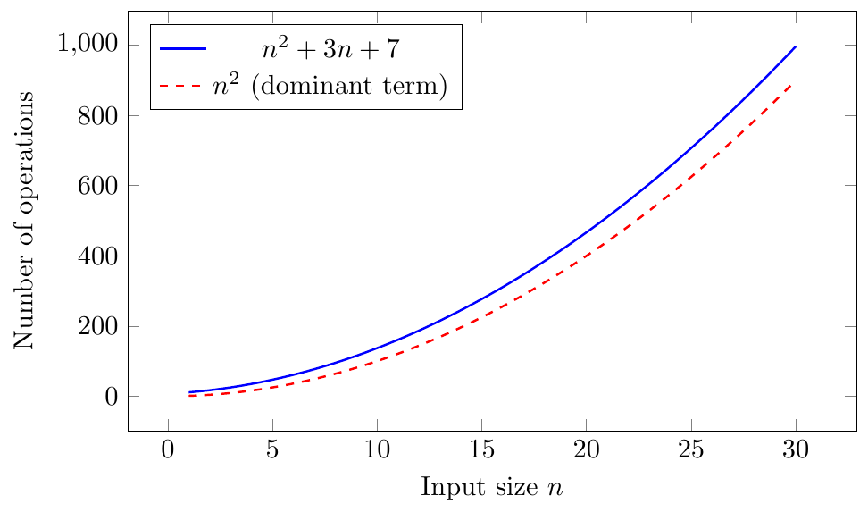
Notice in the graph that the solid curve ($n^2+3n+7$) and the dashed curve ($n^2$) come very close together as $n$ becomes large. This shows visually why we can ignore the smaller terms and constants.
When we compare two algorithms, we do not check their exact step count. We check their order of growth. An algorithm with a slower growing order of growth is better for large input, even if it looks worse for small input.
Suppose Algorithm A takes $5n + 20$ steps, and Algorithm B takes $n^2 + 3n$ steps. Algorithm A grows linearly, and Algorithm B grows quadratically. For small $n$, both may take similar steps. But for large $n$, Algorithm A becomes much faster than Algorithm B, because linear growth is slower than quadratic growth.
Suppose Algorithm A needs $4n + 10$ operations, and Algorithm B needs $n^2$ operations.
Case 1: Small input, $n = 5$ \[ A = 4(5) + 10 = 30, B = 5^2 = 25 \] Here, B is actually doing fewer operations than A.
Case 2: Large input, $n = 1000$ \[ A = 4(1000) + 10 = 4010, B = 1000^2 = 1{,}000{,}000 \] Now, A is doing far fewer operations than B.
This shows that for small input, the algorithm with a worse order of growth can still look better. But as input size grows large, the algorithm with the better order of growth always wins. So, asymptotically, Algorithm A is the better choice.
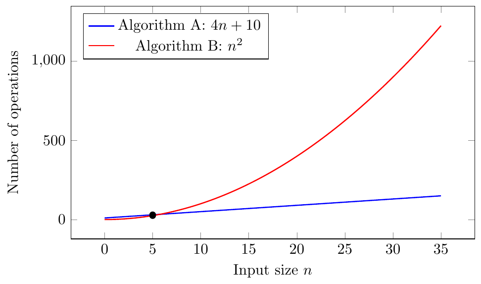
The graph shows the crossover point, where Algorithm B's curve crosses above Algorithm A's curve. Before this point, B looks better. After this point, A is always better, and the gap keeps increasing as $n$ grows.
For each running time expression, identify the dominant term, that means the order of growth.
$T(n) = 7n^3 + 50n^2 + 100$ $\rightarrow$ dominant term is $n^3$
$T(n) = 2^n + n^{10}$ $\rightarrow$ dominant term is $2^n$
$T(n) = 20n \log n + 5n$ $\rightarrow$ dominant term is $n \log n$
$T(n) = n! + 2^n + n^5$ $\rightarrow$ dominant term is $n!$
O-Notation (Big-Oh Notation)
Big-Oh notation gives us an upper bound on how fast a function grows. It tells us that a function $f(n)$ does not grow faster than another function $g(n)$, once $n$ becomes large enough, except for a constant multiplying factor.
Formally, we say $f(n) = O(g(n))$ if we can find two positive numbers $c$ and $n_0$, such that \[ 0 \le f(n) \le c \cdot g(n) \text{for all } n \ge n_0 \]
In simple words, after some point $n_0$, the function $f(n)$ always stays below or on the curve $c \cdot g(n)$. We do not care what happens before $n_0$, we only care about large $n$.
Think of a speed limit board on a highway that says maximum speed is 80. A car may go slow sometimes, fast sometimes, but it never crosses 80, once it is on the highway. Big-Oh is similar, $c \cdot g(n)$ acts like a speed limit, and $f(n)$ never crosses it, after point $n_0$.
Maths intuition: Why do we allow a constant $c$ and a starting point $n_0$?
The constant $c$ is needed because we do not care about exact values, we only care about growth pattern. So even if $f(n)$ is a bit bigger than $g(n)$, like $f(n) = 5g(n)$, we can still say $f(n) = O(g(n))$, by simply choosing $c = 5$ or more.
The point $n_0$ is needed because for small $n$, a function may behave randomly, or one function may be bigger than other by chance. We only care about behavior when $n$ becomes large, so we allow the inequality to fail for small $n$, before $n_0$.
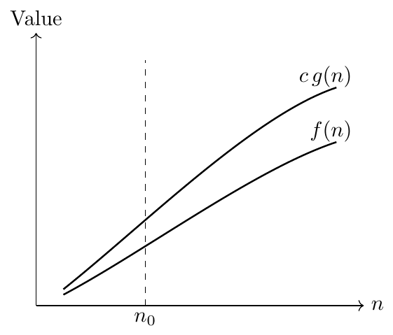
In this picture, before $n_0$, the curve $f(n)$ might cross above $c \cdot g(n)$, that is fine. But after $n_0$, $f(n)$ always stays below $c \cdot g(n)$. This is exactly what the Big-Oh definition demands.
$O(g(n))$ is actually a set of functions, not a single function. Writing $f(n) = O(g(n))$ really means $f(n)$ belongs to this set.
The constants $c$ and $n_0$ are not fixed or unique. Many valid choices of $c$ and $n_0$ can work for the same proof.
Big-Oh ignores small input behavior. Only what happens as $n$ becomes very large matters.
A slower growing function can still belong to a faster growing function's class. For example, $n \in O(n^2)$, because $n$ never grows faster than $n^2$. This does not mean they grow at the same rate, it only means $n$ does not cross $n^2$ beyond a constant factor.
We assume $f(n)$ is non-negative for large $n$, so that the comparison $f(n) \le c \cdot g(n)$ makes proper sense.
We want to show $f(n) = O(n)$.
We need to find $c > 0$ and $n_0$ such that \[ 0 \le 3n + 8 \le c \cdot n \text{for all } n \ge n_0 \]
For $n \ge 8$, we know $8 \le n$. So, \[ 3n + 8 \le 3n + n = 4n \]
This means $3n + 8 \le 4n$ for all $n \ge 8$.
Choosing $c = 4$ and $n_0 = 8$, the condition holds. So, \[ 3n + 8 = O(n) \]
We want to show $f(n) = O(n^2)$.
We need $c > 0$ and $n_0$ such that \[ 0 \le n^2 + 1 \le c \cdot n^2 \text{for all } n \ge n_0 \]
For $n \ge 1$, we know $1 \le n^2$. So, \[ n^2 + 1 \le n^2 + n^2 = 2n^2 \]
This means $n^2 + 1 \le 2n^2$ for all $n \ge 1$.
Choosing $c = 2$ and $n_0 = 1$, the condition holds. So, \[ n^2 + 1 = O(n^2) \]
We want to show $f(n) = O(n^2)$.
For $n \ge 5$, we know $5 \le n$. So, \[ 100n + 5 \le 100n + n = 101n \]
Also, for $n \ge 1$, we know $n \le n^2$, so $101n \le 101n^2$.
Combining, for $n \ge 5$, \[ 100n + 5 \le 101n^2 \]
Choosing $c = 101$ and $n_0 = 5$, the condition holds. So, \[ 100n + 5 = O(n^2) \]
Prove that $f(n) = O(n^2)$.
Solution: For $n \ge 1$, we know $3n \le 3n^2$. So, \[ 5n^2 + 3n \le 5n^2 + 3n^2 = 8n^2 \] Choosing $c = 8$ and $n_0 = 1$, we get $5n^2 + 3n = O(n^2)$.
Prove that $f(n) = O(n^3)$.
Solution: For $n \ge 50$, we know $50n^2 \le n \cdot n^2 = n^3$. So, \[ n^3 + 50n^2 \le n^3 + n^3 = 2n^3 \] Choosing $c = 2$ and $n_0 = 50$, we get $n^3 + 50n^2 = O(n^3)$.
Prove that $f(n) = O(1)$.
Solution: Here $f(n) = 7$ stays fixed, it does not grow with $n$. So, \[ 7 \le 7 \cdot 1 \] Choosing $c = 7$ and $n_0 = 1$, we get $7 = O(1)$. This shows constant functions are written as $O(1)$.
Prove that $f(n) = O(n \log n)$.
Solution: For $n \ge 2$, we know $\log n \ge 1$, so $n \le n \log n$. So, \[ n \log n + n \le n \log n + n \log n = 2 n \log n \] Choosing $c = 2$ and $n_0 = 2$, we get $n \log n + n = O(n \log n)$.
Prove that $f(n) = O(n^2)$.
Solution: For $n \ge 2$, we know $\log n \le n$, so $3n \log n \le 3n^2$. Also for $n \ge 1$, $10 \le 10n^2$. So, \[ 2n^2 + 3n \log n + 10 \le 2n^2 + 3n^2 + 10n^2 = 15n^2 \] Choosing $c = 15$ and $n_0 = 2$, we get $2n^2 + 3n \log n + 10 = O(n^2)$.
$\Omega$-Notation (Big-Omega Notation)
Big-Omega notation gives us a lower bound on how fast a function grows. It tells us that a function $f(n)$ grows at least as fast as another function $g(n)$, once $n$ becomes large enough, except for a constant multiplying factor.
Formally, we say $f(n) = \Omega(g(n))$ if we can find two positive numbers $c$ and $n_0$, such that \[ 0 \le c \cdot g(n) \le f(n) \text{for all } n \ge n_0 \]
In simple words, after some point $n_0$, the function $f(n)$ always stays above or on the curve $c \cdot g(n)$. We do not care what happens before $n_0$, we only care about large $n$.
Think of a rule that says a worker must be paid at least 500 rupees per day. The actual pay can be more, some days much more, but it never falls below this floor amount. Big-Omega is similar, $c \cdot g(n)$ acts like a floor, and $f(n)$ never falls below it, after point $n_0$.
Maths intuition: Big-Oh and Big-Omega are like opposite directions of the same idea.
In Big-Oh, $f(n)$ stays below $c \cdot g(n)$, so $g(n)$ acts as a ceiling.
In Big-Omega, $f(n)$ stays above $c \cdot g(n)$, so $g(n)$ acts as a floor.
The constant $c$ lets us shrink $g(n)$ a little, so even if $f(n)$ is somewhat smaller than $g(n)$, we can still find a smaller version of $g(n)$ that $f(n)$ stays above.
The point $n_0$ lets us ignore small $n$, where the inequality might not hold by chance.
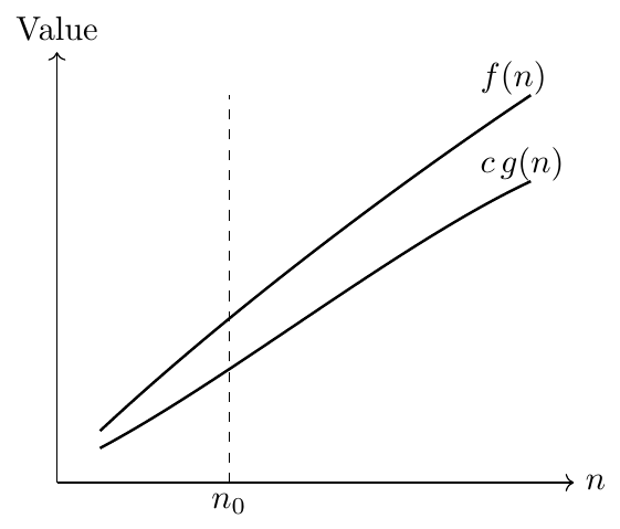
In this picture, after $n_0$, the curve $f(n)$ always stays above $c \cdot g(n)$. Before $n_0$, this may or may not be true, and we do not worry about that part.
$\Omega(g(n))$ is a set of functions, not a single function. Writing $f(n) = \Omega(g(n))$ means $f(n) \in \Omega(g(n))$.
The constants $c$ and $n_0$ are not fixed or unique. Many valid pairs can work for the same proof.
Only behavior as $n \to \infty$ matters. Small input values are ignored.
If $f(n)$ grows faster than $g(n)$, then $f(n)$ can still belong to $\Omega(g(n))$. For example, $n^2 \in \Omega(n)$, because $n^2$ eventually grows at least as fast as $n$. This does not mean they grow at the same rate, it only means $n^2$ never falls below $n$, up to a constant factor.
We assume $f(n)$ and $g(n)$ are non-negative for large $n$, so the comparison makes proper sense.
We want to show $f(n) = \Omega(n^2)$.
We need $c > 0$ and $n_0$ such that \[ 0 \le c \cdot n^2 \le 3n^2 + 2n \text{for all } n \ge n_0 \]
Since $2n \ge 0$ for all $n \ge 0$, \[ 3n^2 + 2n \ge 3n^2 \]
This means $3n^2 + 2n \ge 3n^2$ for all $n \ge 0$.
Choosing $c = 3$ and $n_0 = 1$, the condition holds. So, \[ 3n^2 + 2n = \Omega(n^2) \]
Prove that $f(n) = \Omega(n^2)$.
Solution: For $n \ge 6$, we know $3n \le \dfrac{1}{2}n^2$. So, \[ n^2 - 3n \ge n^2 - \frac{1}{2}n^2 = \frac{1}{2}n^2 \] Choosing $c = \dfrac{1}{2}$ and $n_0 = 6$, we get $n^2 - 3n = \Omega(n^2)$.
Prove that $f(n) = \Omega(n)$.
Solution: Since $2 \ge 0$ for all $n$, \[ 7n + 2 \ge 7n \] Choosing $c = 7$ and $n_0 = 1$, we get $7n + 2 = \Omega(n)$.
Prove that $f(n) = \Omega(n^3)$.
Solution: Since $4n \ge 0$ for all $n \ge 0$, \[ n^3 + 4n \ge n^3 \] Choosing $c = 1$ and $n_0 = 1$, we get $n^3 + 4n = \Omega(n^3)$.
Prove that $f(n) = \Omega(n)$.
Solution: For $n \ge 2$, we know $\log n \ge 1$. So, \[ n \log n \ge n \cdot 1 = n \] Choosing $c = 1$ and $n_0 = 2$, we get $n \log n = \Omega(n)$.
Prove that $f(n) = \Omega(n^2)$.
Solution: It is known that $2^n$ grows much faster than any polynomial like $n^2$, for large $n$. We can check small values to find a safe starting point. At $n = 6$, $2^n = 64$ and $n^2 = 36$, so $2^n \ge n^2$ here. As $n$ increases further, $2^n$ grows much faster than $n^2$, so the inequality keeps holding. \[ 2^n \ge n^2 \text{for all } n \ge 6 \] Choosing $c = 1$ and $n_0 = 6$, we get $2^n = \Omega(n^2)$.
$\Theta$-Notation (Big-Theta Notation)
Big-Theta notation gives us a tight bound on how fast a function grows. It tells us that a function $f(n)$ grows neither faster nor slower than $g(n)$, once $n$ becomes large enough, except for constant factors. This means $f(n)$ and $g(n)$ grow at the same rate.
Formally, we say $f(n) = \Theta(g(n))$ if we can find three positive numbers $c_1$, $c_2$, and $n_0$, such that \[ 0 \le c_1 \cdot g(n) \le f(n) \le c_2 \cdot g(n) \text{for all } n \ge n_0 \]
In simple words, after some point $n_0$, the function $f(n)$ is always sandwiched between $c_1 \cdot g(n)$ and $c_2 \cdot g(n)$. It never goes too high above $g(n)$, and never goes too low below $g(n)$.
Think of a narrow road with a wall on the left side and a wall on the right side. A car driving on this road can never go beyond the left wall, and can never go beyond the right wall, it always stays between them. Big-Theta is similar, $f(n)$ always stays between the lower wall $c_1 \cdot g(n)$ and the upper wall $c_2 \cdot g(n)$.
Maths intuition: Big-Theta is simply Big-Oh and Big-Omega combined together.
Big-Oh alone tells us $f(n)$ does not grow faster than $g(n)$, that is an upper bound only.
Big-Omega alone tells us $f(n)$ does not grow slower than $g(n)$, that is a lower bound only.
Big-Theta needs both conditions to be true at the same time. So if we already know $f(n) = O(g(n))$ and $f(n) = \Omega(g(n))$, then automatically $f(n) = \Theta(g(n))$.
This is the strongest and most informative notation, because it tells us the exact growth class of $f(n)$, not just an upper limit or just a lower limit.
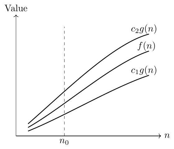
In this picture, after $n_0$, the function $f(n)$ is trapped between the lower curve $c_1 g(n)$ and the upper curve $c_2 g(n)$. This trapped region is the visual meaning of Big-Theta.
$\Theta(g(n))$ is a set of functions, not a single function. Writing $f(n) = \Theta(g(n))$ means $f(n) \in \Theta(g(n))$.
Big-Theta needs two inequalities together, $c_1 g(n) \le f(n)$ and $f(n) \le c_2 g(n)$. Both must be true at the same time, for the same $n_0$.
Only behavior for large $n$ matters. Small $n$ does not affect membership in $\Theta(g(n))$.
Constant multiplying factors do not change the Theta class. For example, $a n^2 \in \Theta(n^2)$, for any positive constant $a$.
If $f(n) = \Theta(g(n))$, then $f(n)$ and $g(n)$ grow at the same speed, neither one beats the other by more than a constant factor, as $n$ becomes large.
We want to show $f(n) = \Theta(n^2)$.
Step 1: Upper Bound. For $n \ge 1$, we know $3n \le 3n^2$ and $4 \le 4n^2$. So, \[ f(n) \le 2n^2 + 3n^2 + 4n^2 = 9n^2 \] This gives us $c_2 = 9$.
Step 2: Lower Bound. Since all terms in $f(n)$ are non-negative for $n \ge 1$, \[ f(n) \ge 2n^2 \] This gives us $c_1 = 2$.
Step 3: Combine. For all $n \ge 1$, \[ 2n^2 \le 2n^2 + 3n + 4 \le 9n^2 \]
Choosing $c_1 = 2$, $c_2 = 9$, and $n_0 = 1$, both conditions hold together. So, \[ 2n^2 + 3n + 4 = \Theta(n^2) \]
Prove that $f(n) = \Theta(n)$.
Upper bound: For $n \ge 1$, $5n + 2 \le 5n + 2n = 7n$, so $c_2 = 7$.
Lower bound: Since $2 \ge 0$, $5n + 2 \ge 5n$, so $c_1 = 5$.
Choosing $c_1 = 5$, $c_2 = 7$, $n_0 = 1$, we get $5n + 2 = \Theta(n)$.
Prove that $f(n) = \Theta(n^2)$.
Upper bound: For $n \ge 1$, $n \le n^2$, so $n^2 + n \le n^2 + n^2 = 2n^2$, giving $c_2 = 2$.
Lower bound: Since $n \ge 0$, $n^2 + n \ge n^2$, giving $c_1 = 1$.
Choosing $c_1 = 1$, $c_2 = 2$, $n_0 = 1$, we get $n^2 + n = \Theta(n^2)$.
Prove that $f(n) = \Theta(n^3)$.
Upper bound: For $n \ge 1$, $2n^2 \le 2n^3$ and $n \le n^3$, so \[ f(n) \le 3n^3 + 2n^3 + n^3 = 6n^3, c_2 = 6 \]
Lower bound: Since all terms are non-negative, $f(n) \ge 3n^3$, so $c_1 = 3$.
Choosing $c_1 = 3$, $c_2 = 6$, $n_0 = 1$, we get $3n^3 + 2n^2 + n = \Theta(n^3)$.
Prove that $f(n) = \Theta(n^2)$.
Lower bound: For $n \ge 12$, $3n \le \dfrac{1}{4}n^2$, so \[ f(n) \ge \frac{1}{2}n^2 - \frac{1}{4}n^2 = \frac{1}{4}n^2, c_1 = \frac{1}{4} \]
Upper bound: Since $3n \ge 0$ does not add value here, simply $f(n) \le \dfrac{1}{2}n^2$, so $c_2 = \dfrac{1}{2}$.
Choosing $c_1 = \dfrac{1}{4}$, $c_2 = \dfrac{1}{2}$, $n_0 = 12$, we get $\dfrac{1}{2}n^2 - 3n = \Theta(n^2)$.
Prove that $f(n) = \Theta(n \log n)$.
Upper bound: For $n \ge 2$, $\log n \ge 1$, so $n \le n \log n$, giving \[ f(n) \le n \log n + n \log n = 2n \log n, c_2 = 2 \]
Lower bound: Since $n \ge 0$, $f(n) \ge n \log n$, giving $c_1 = 1$.
Choosing $c_1 = 1$, $c_2 = 2$, $n_0 = 2$, we get $n \log n + n = \Theta(n \log n)$.
Relationship Between $O$, $\Omega$, and $\Theta$
Big-Oh, Big-Omega, and Big-Theta are not separate, unrelated ideas. They are connected to each other through some simple rules. These rules help us prove one notation using another, and help us understand them better as a single family.
If $f(n) = \Theta(g(n))$, and $g(n) = \Theta(h(n))$, then $f(n) = \Theta(h(n))$. This same rule also works for $O$ and $\Omega$. In simple words, if $A$ matches $B$ in growth, and $B$ matches $C$ in growth, then $A$ also matches $C$ in growth.
If Ravi is as tall as Suresh, and Suresh is as tall as Mahesh, then Ravi is also as tall as Mahesh. Transitivity in notations works the same way, just with growth rate instead of height.
Any function is always related to itself in the same notation. That means $f(n) = O(f(n))$. This same rule works for $\Theta$ and $\Omega$ also. In simple words, a function always grows at the same rate as itself, which is obviously true.
This rule is only for Big-Theta. $f(n) = \Theta(g(n))$ if and only if $g(n) = \Theta(f(n))$. In simple words, if $f(n)$ grows at the same rate as $g(n)$, then $g(n)$ also grows at the same rate as $f(n)$. This makes sense because Big-Theta means equal growth, and equal growth works both ways.
This rule connects Big-Oh and Big-Omega together. $f(n) = O(g(n))$ if and only if $g(n) = \Omega(f(n))$. In simple words, if $f(n)$ does not grow faster than $g(n)$, then automatically $g(n)$ does not grow slower than $f(n)$. These are just two ways of saying the same thing, from different sides.
For any two functions $f(n)$ and $g(n)$ that stay non-negative for large $n$, \[ f(n) = \Theta(g(n)) \text{if and only if} f(n) = O(g(n)) \text{ and } f(n) = \Omega(g(n)) \] This means, to prove Big-Theta, we do not need a brand new method. We simply prove Big-Oh first, then prove Big-Omega separately, and if both are true, Big-Theta is automatically true.
Think back to the road between two walls example used for Big-Theta. The left wall is the lower bound, which is Big-Omega. The right wall is the upper bound, which is Big-Oh. If we show the car never crosses the left wall, and never crosses the right wall, we have shown the car always stays on this road, which is exactly Big-Theta.
We want to show that for $a > 0$, $f(n) = an^2 + bn + c = \Theta(n^2)$.
Step 1: Prove Big-Oh. For $n \ge 1$, we know $|bn| \le |b| n^2$ and $|c| \le |c| n^2$. So, \[ f(n) \le an^2 + |b|n^2 + |c|n^2 = (a + |b| + |c|) n^2 \] This shows $f(n) = O(n^2)$.
Step 2: Prove Big-Omega. Since $a > 0$, the term $an^2$ is the strongest term, and it grows faster than $bn$ and $c$. So, for large enough $n$, the smaller terms cannot pull the value below half of $an^2$. There exists some $n_0$ such that \[ an^2 + bn + c \ge \frac{a}{2} n^2 \text{for all } n \ge n_0 \] This shows $f(n) = \Omega(n^2)$.
Step 3: Combine. Since $f(n)$ is both $O(n^2)$ and $\Omega(n^2)$, by the rule connecting the three notations, \[ an^2 + bn + c = \Theta(n^2) \]
Given $f(n) = \Theta(n^2)$ and $g(n) = \Theta(n^2)$, with $h(n) = n^2$, show $f(n) = \Theta(h(n))$.
Solution: Since $f(n) = \Theta(g(n))$, and $g(n) = \Theta(h(n))$ (because both $g(n)$ and $h(n)$ are $\Theta(n^2)$), by transitivity, $f(n) = \Theta(h(n))$.
Given $n = O(n^2)$, what can we say about $n^2$ using transpose symmetry?
Solution: By transpose symmetry, since $n = O(n^2)$, it directly follows that $n^2 = \Omega(n)$.
Show that $f(n) = 4n^2 - 5n$ is $\Theta(n^2)$.
Upper bound: For $n \ge 1$, $f(n) \le 4n^2$, so $f(n) = O(n^2)$.
Lower bound: For $n \ge 3$, $5n \le 2n^2$, so $f(n) \ge 4n^2 - 2n^2 = 2n^2$, giving $f(n) = \Omega(n^2)$.
Since both hold, $f(n) = \Theta(n^2)$.
If $5n^2 = \Theta(n^2)$, what can we say about $n^2$ in relation to $5n^2$?
Solution: By symmetry of Big-Theta, since $5n^2 = \Theta(n^2)$, it directly follows that $n^2 = \Theta(5n^2)$.
Given $n \log n = \Theta(n \log n)$, and $n \log n = \Theta(2n \log n)$, and $2n \log n = \Theta(3n \log n)$, what can we conclude about $n \log n$ and $3n \log n$?
Solution: Using transitivity twice, since $n \log n = \Theta(2n \log n)$ and $2n \log n = \Theta(3n \log n)$, we get $n \log n = \Theta(3n \log n)$.
Little-$o$ Notation
Little-$o$ notation also gives an upper bound, like Big-Oh. But there is a big difference. In Big-Oh, $f(n)$ can grow at the same rate as $g(n)$. In little-$o$, $f(n)$ must grow strictly slower than $g(n)$, not at the same rate.
Formally, we say $f(n) = o(g(n))$ if, for every positive constant $c$, no matter how small, we can find a value $n_0$ such that \[ 0 \le f(n) < c \cdot g(n) \text{for all } n \ge n_0 \]
The key difference from Big-Oh is this, in little-$o$, the inequality must hold for every possible $c > 0$, even very tiny values of $c$, not just for some one fixed $c$.
Think of two brothers walking. Big-Oh is like saying the younger brother never walks faster than the older brother, but they could be walking at the exact same speed. Little-$o$ is like saying the younger brother always walks strictly slower, he can never catch up to the same speed, no matter how slow we let the older brother go.
Little-$o$ gives a strict upper bound, meaning $f(n)$ grows strictly slower than $g(n)$.
Unlike Big-Oh, here the condition must hold for every $c > 0$, not just one specific $c$. This makes little-$o$ a stronger and more demanding condition than Big-Oh.
If $f(n) = o(g(n))$, then automatically $f(n) = O(g(n))$ also holds. But the opposite is not always true.
A function is never little-$o$ of itself. That means $f(n) \ne o(f(n))$, because $f(n)$ cannot grow strictly slower than itself.
A simple way to check little-$o$ is using limits, \[ \lim_{n \to \infty} \frac{f(n)}{g(n)} = 0 \] If this limit becomes exactly $0$, then $f(n) = o(g(n))$.
We check whether $n = o(n^2)$, using the limit method. \[ \lim_{n \to \infty} \frac{n}{n^2} = \lim_{n \to \infty} \frac{1}{n} = 0 \] Since the limit is $0$, we conclude \[ n = o(n^2) \] This makes sense, because $n$ grows much slower than $n^2$, as $n$ becomes large.
We check whether $n^2 = o(n^2)$. \[ \lim_{n \to \infty} \frac{n^2}{n^2} = 1 \] Since the limit is $1$, not $0$, we conclude \[ n^2 \ne o(n^2) \] This confirms that little-$o$ does not allow same speed growth, only strictly slower growth is allowed.
Little-$\omega$ Notation
Little-$\omega$ notation gives a lower bound, like Big-Omega. But just like little-$o$, there is a strictness added here. In Big-Omega, $f(n)$ can grow at the same rate as $g(n)$. In little-$\omega$, $f(n)$ must grow strictly faster than $g(n)$, not at the same rate.
Formally, we say $f(n) = \omega(g(n))$ if, for every positive constant $c$, no matter how large, we can find a value $n_0$ such that \[ 0 \le c \cdot g(n) < f(n) \text{for all } n \ge n_0 \]
Here also, the condition must hold for every possible $c > 0$, not just one fixed $c$, which makes little-$\omega$ a stronger condition than Big-Omega.
Think of a runner who is always strictly faster than another runner, no matter how much we slow down the comparison runner. This is little-$\omega$, a strict, always faster relationship. Big-Omega only says our runner is never slower, they could even run at the same speed sometimes.
Little-$\omega$ gives a strict lower bound, meaning $f(n)$ grows strictly faster than $g(n)$.
The condition must hold for every $c > 0$, not just one specific $c$, making it stronger than Big-Omega.
If $f(n) = \omega(g(n))$, then automatically $f(n) = \Omega(g(n))$ also holds. But the opposite is not always true.
A function is never little-$\omega$ of itself, since $f(n)$ cannot grow strictly faster than itself.
A simple way to check little-$\omega$ is using limits, \[ \lim_{n \to \infty} \frac{f(n)}{g(n)} = \infty \] If this limit becomes infinity, then $f(n) = \omega(g(n))$.
Little-$o$ and little-$\omega$ are reverse of each other, just like Big-Oh and Big-Omega. If $f(n) = o(g(n))$, then $g(n) = \omega(f(n))$.
We check whether $n^2 = \omega(n)$, using the limit method. \[ \lim_{n \to \infty} \frac{n^2}{n} = \lim_{n \to \infty} n = \infty \] Since the limit is infinity, we conclude \[ n^2 = \omega(n) \] This makes sense, because $n^2$ grows much faster than $n$, as $n$ becomes large.
We check whether $2^n = \omega(n^{10})$. \[ \lim_{n \to \infty} \frac{2^n}{n^{10}} = \infty \] This is true because exponential growth always beats polynomial growth, eventually, no matter how large the power is. So, \[ 2^n = \omega(n^{10}) \]
Check whether $\log n = o(n)$.
Solution: \[ \lim_{n \to \infty} \frac{\log n}{n} = 0 \] Since the limit is $0$, we get $\log n = o(n)$.
Check whether $n^3 = o(n^2)$.
Solution: \[ \lim_{n \to \infty} \frac{n^3}{n^2} = \lim_{n \to \infty} n = \infty \] Since the limit is not $0$, we get $n^3 \ne o(n^2)$. In fact, $n^3 = \omega(n^2)$ instead.
Check whether $n! = \omega(2^n)$.
Solution: As $n$ becomes large, factorial growth becomes much faster than exponential growth. \[ \lim_{n \to \infty} \frac{n!}{2^n} = \infty \] So, $n! = \omega(2^n)$.
Check whether $5n^2 = o(n^2)$.
Solution: \[ \lim_{n \to \infty} \frac{5n^2}{n^2} = 5 \] Since the limit is a fixed constant, not $0$, we get $5n^2 \ne o(n^2)$. Instead, $5n^2 = \Theta(n^2)$.
Check whether $n \log n = \omega(n)$.
Solution: \[ \lim_{n \to \infty} \frac{n \log n}{n} = \lim_{n \to \infty} \log n = \infty \] Since the limit is infinity, we get $n \log n = \omega(n)$.
Relationship Between $O$, $\Omega$, $\Theta$, $o$, and $\omega$
We can group all five notations into two families. One family compares growth allowing equal growth also, this is the non-strict family, containing $O$, $\Omega$, and $\Theta$. The other family compares growth not allowing equal growth, this is the strict family, containing $o$ and $\omega$. Little-$o$ is the strict version of Big-Oh, and little-$\omega$ is the strict version of Big-Omega. There is no strict version of Big-Theta, because Theta already means exact equal growth.
Think of two ways to compare numbers. We can say $a \le b$, which allows $a$ to be equal to $b$. Or we can say $a < b$, which does not allow them to be equal. Big-Oh is like $\le$, and little-$o$ is like $<$. The same pattern goes for Big-Omega and little-$\omega$.
All five notations can be checked using the limit \[ L = \lim_{n \to \infty} \frac{f(n)}{g(n)} \] Depending on the value of $L$, we know which notation applies.
If $L = 0$, then $f(n) = o(g(n))$, and also $f(n) = O(g(n))$.
If $L$ is a positive finite constant, then $f(n) = \Theta(g(n))$, and also $f(n) = O(g(n))$ and $f(n) = \Omega(g(n))$.
If $L = \infty$, then $f(n) = \omega(g(n))$, and also $f(n) = \Omega(g(n))$.
This single limit test tells us exactly which notations are true and which are false, for a given pair $f(n)$ and $g(n)$.
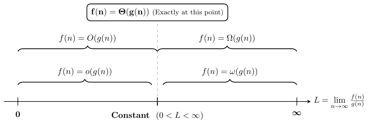
$f(n) = o(g(n))$ always implies $f(n) = O(g(n))$, because strictly slower also means not faster. But $O$ does not imply $o$, since $O$ allows equal growth also.
$f(n) = \omega(g(n))$ always implies $f(n) = \Omega(g(n))$, because strictly faster also means not slower. But $\Omega$ does not imply $\omega$, since $\Omega$ allows equal growth also.
$f(n) = \Theta(g(n))$ if and only if both $f(n) = O(g(n))$ and $f(n) = \Omega(g(n))$ are true together.
$f(n) = o(g(n))$ and $f(n) = \omega(g(n))$ can never both be true for the same pair $f(n)$ and $g(n)$, because one says strictly slower and other says strictly faster, they cannot both happen.
$f(n) = o(g(n))$ and $f(n) = \Theta(g(n))$ can never both be true together, because $o$ means strictly slower, but $\Theta$ means equal growth.
Just like $f(n) = O(g(n))$ if and only if $g(n) = \Omega(f(n))$, the same flipping rule works for the strict family also. $f(n) = o(g(n))$ if and only if $g(n) = \omega(f(n))$. For example, since $n = o(n^2)$, by this flipping rule, we directly get $n^2 = \omega(n)$, without checking the limit again.
The big notations ($O$, $\Omega$, $\Theta$) and the little notations ($o$, $\omega$) are not independent, they sit inside each other in a strict-inside-non-strict pattern.
Every function pair classified by $o$ is automatically also classified by $O$. So $o(g(n))$ is a smaller, stricter set sitting entirely inside $O(g(n))$.
Every function pair classified by $\omega$ is automatically also classified by $\Omega$. So $\omega(g(n))$ sits entirely inside $\Omega(g(n))$.
$O(g(n))$ can be split into exactly two non-overlapping parts: the part where growth is strictly slower, which is $o(g(n))$, and the part where growth is exactly equal, which is $\Theta(g(n))$. That is, \[ O(g(n)) = o(g(n)) \cup \Theta(g(n)) \]
Similarly, $\Omega(g(n))$ splits into $\omega(g(n))$ and $\Theta(g(n))$: \[ \Omega(g(n)) = \omega(g(n)) \cup \Theta(g(n)) \]
Because of this split, if we already know $f(n) = O(g(n))$ but we can rule out $f(n) = \Theta(g(n))$, we can directly conclude the stronger fact $f(n) = o(g(n))$. The same logic applies to $\Omega$ and $\omega$.
We already know from Practice 1 that $f(n) = O(n^3)$. Now check whether $f(n) = \Theta(n^3)$ is true. Since \[ \lim_{n \to \infty} \frac{n^2}{n^3} = 0 \ne \text{positive constant} \] $\Theta$ is ruled out. Since $O(g(n)) = o(g(n)) \cup \Theta(g(n))$, and $\Theta$ is ruled out, we directly conclude \[ f(n) = o(n^3) \] without needing to separately confirm the strict limit condition.
The strict notations are transitive. If $f(n) = o(g(n))$ and $g(n) = o(h(n))$, then \[ f(n) = o(h(n)) \] Similarly, if $f(n) = \omega(g(n))$ and $g(n) = \omega(h(n))$, then \[ f(n) = \omega(h(n)) \] Think of it as a chain of strictly-slower-than relationships. If $A$ is strictly slower than $B$, and $B$ is strictly slower than $C$, then $A$ must be strictly slower than $C$ as well, the strictness carries through the whole chain.
We know $\log n = o(n)$, and we know $n = o(n^2)$. By transitivity of $o$, without computing any new limit, we can directly conclude \[ \log n = o(n^2) \] By the transpose symmetry rule, this also tells us $n^2 = \omega(\log n)$.
\[ \lim_{n \to \infty} \frac{3n^2}{n^2} = 3 \] The limit is a positive constant, so $f(n) = \Theta(n^2)$. This also means $f(n) = O(n^2)$ and $f(n) = \Omega(n^2)$ are both true. But $f(n) \ne o(n^2)$ and $f(n) \ne \omega(n^2)$, since the limit is not $0$ and not $\infty$.
\[ \lim_{n \to \infty} \frac{n \log n}{n^2} = \lim_{n \to \infty} \frac{\log n}{n} = 0 \] The limit is $0$, so $f(n) = o(n^2)$. This also means $f(n) = O(n^2)$ is true. But $f(n) \ne \Theta(n^2)$, $f(n) \ne \Omega(n^2)$, and $f(n) \ne \omega(n^2)$.
Find the limit and classify the relationship.
Solution: \[ \lim_{n \to \infty} \frac{n^2}{n^3} = 0 \] So, $f(n) = o(n^3)$, which also means $f(n) = O(n^3)$.
Find the limit and classify the relationship.
Solution: \[ \lim_{n \to \infty} \frac{2^n}{3^n} = \lim_{n \to \infty} \left(\frac{2}{3}\right)^n = 0 \] So, $f(n) = o(3^n)$, which also means $f(n) = O(3^n)$.
Find the limit and classify the relationship.
Solution: Since $n^n$ multiplies $n$ copies of $n$, but $n!$ multiplies decreasing numbers below $n$, $n^n$ grows faster. \[ \lim_{n \to \infty} \frac{n!}{n^n} = 0 \] So, $f(n) = o(n^n)$, which also means $f(n) = O(n^n)$.
Find the limit and classify the relationship.
Solution: \[ \lim_{n \to \infty} \frac{7n^2 + 2n}{n^2} = 7 \] Since the limit is a positive constant, $f(n) = \Theta(n^2)$, which also means $f(n) = O(n^2)$ and $f(n) = \Omega(n^2)$.
Find the limit and classify the relationship.
Solution: \[ \lim_{n \to \infty} \frac{n^3}{n^2 \log n} = \lim_{n \to \infty} \frac{n}{\log n} = \infty \] So, $f(n) = \omega(n^2 \log n)$, which also means $f(n) = \Omega(n^2 \log n)$.
When two functions are added together, the sum is bounded by whichever growth rate is faster. Formally, if $f_1(n) = O(g_1(n))$ and $f_2(n) = O(g_2(n))$, then \[ f_1(n) + f_2(n) = O\big(\max(g_1(n), g_2(n))\big) \] The same idea holds for $\Omega$: if $f_1(n) = \Omega(g_1(n))$ and $f_2(n) = \Omega(g_2(n))$, then $f_1(n) + f_2(n) = \Omega\big(\max(g_1(n), g_2(n))\big)$.
A useful special case, often called the Max Rule, applies when $f(n)$ and $g(n)$ are both asymptotically non-negative: \[ f(n) + g(n) = \Theta\big(\max(f(n), g(n))\big) \] The intuition is simple: when you add a slow-growing term to a fast-growing term, the slow term eventually becomes insignificant, so the sum behaves like the faster term alone.
Here the two terms are $n^3$ and $n^2 \log n$. Since $n^3$ grows faster than $n^2 \log n$, the max rule tells us \[ n^3 + n^2 \log n = \Theta(n^3) \] We do not need to analyze both terms separately in later steps of an algorithm's analysis; only the dominant term $n^3$ matters for the overall growth rate.
When two functions are multiplied, their bounds multiply together as well. If $f_1(n) = O(g_1(n))$ and $f_2(n) = O(g_2(n))$, then \[ f_1(n) \cdot f_2(n) = O\big(g_1(n) \cdot g_2(n)\big) \] The same pattern holds for $\Omega$ and $\Theta$:
If $f_1(n) = \Omega(g_1(n))$ and $f_2(n) = \Omega(g_2(n))$, then $f_1(n) \cdot f_2(n) = \Omega(g_1(n) \cdot g_2(n))$.
If $f_1(n) = \Theta(g_1(n))$ and $f_2(n) = \Theta(g_2(n))$, then $f_1(n) \cdot f_2(n) = \Theta(g_1(n) \cdot g_2(n))$.
This property is especially useful when analyzing nested loops, since the work done by an outer loop and an inner loop multiplies together.
Suppose an outer loop runs $\Theta(n)$ times, and for each outer iteration, an inner loop runs $\Theta(\log n)$ times. Treating these as $f_1(n) = \Theta(n)$ and $f_2(n) = \Theta(\log n)$, the product rule gives the total work as \[ f_1(n) \cdot f_2(n) = \Theta(n \log n) \] This is exactly why we multiply the bounds of nested loops instead of adding them.
Multiplying a function by a fixed positive constant does not change its asymptotic classification. If $f(n) = O(g(n))$, then for any constant $c > 0$, \[ c \cdot f(n) = O(g(n)) \] The same holds for $\Omega$, $\Theta$, $o$, and $\omega$. This is why constant factors are always dropped when we state a growth rate, since $2n$, $50n$, and $0.001n$ are all $\Theta(n)$.
Suppose an algorithm performs $5n^2 + 3n$ operations. Using the sum rule, this is $\Theta(n^2)$. Using the constant multiple property, we also see that a related algorithm performing $500n^2$ operations, or even $0.5n^2$ operations, is still $\Theta(n^2)$. Only the shape of growth matters, not the constant in front of it.
Given $f(n) = n \log n$ and $g(n) = n^2$, we already know $f(n) = O(n^2)$. Use the big-little split to decide whether $f(n) = o(n^2)$.
Solution: Check if $\Theta$ holds: \[ \lim_{n \to \infty} \frac{n \log n}{n^2} = 0 \ne \text{positive constant} \] $\Theta$ is ruled out, so since $O(g(n)) = o(g(n)) \cup \Theta(g(n))$, we conclude $f(n) = o(n^2)$.
Given $n^2 = \omega(n \log n)$ and $n \log n = \omega(n)$, what can we conclude?
Solution: By transitivity of $\omega$, \[ n^2 = \omega(n) \]
Classify $f(n) = 2^n + n^{100}$ using the max rule.
Solution: Since $2^n$ grows faster than any polynomial, including $n^{100}$, \[ 2^n + n^{100} = \Theta(2^n) \]
An algorithm has an outer loop of $\Theta(n^2)$ iterations, and inside each iteration it calls a subroutine that costs $\Theta(n)$. Find the total cost.
Solution: By the product rule, \[ \Theta(n^2) \cdot \Theta(n) = \Theta(n^3) \]
Best Case, Worst Case and Average Case
For many algorithms, the running time does not stay fixed, it changes depending on the actual input given, even if the input size $n$ is the same. So, we study three different cases to fully understand the algorithm's behavior, best case, worst case, and average case.
Suppose we are searching for our friend in a queue of people, by checking one by one from the front. If our friend is the first person, we find them fast. If our friend is the last person, we take a long time. If our friend can be anywhere with equal chance, the time taken on average lies somewhere in between.
Worst case means the input that makes the algorithm take the maximum possible time, among all inputs of the same size $n$. We study worst case because it gives us a guarantee, the algorithm will never take more time than this, no matter what input comes.
Suppose we search for a target value in an array of $n$ elements, using linear search, checking one by one. The worst case happens when the target is at the last position, or the target is not present at all in the array. In this case, the algorithm has to check all $n$ elements, so the worst case time is $\Theta(n)$.
Best case means the input that makes the algorithm take the minimum possible time, among all inputs of the same size $n$. Best case is less useful for guarantees, because we cannot expect lucky input every time, but it tells us the fastest the algorithm can ever be.
In the same linear search example, the best case happens when the target is found at the very first position. Here, the algorithm only checks one element, so the best case time is $\Theta(1)$.
Average case means the expected time taken by the algorithm, averaged over all possible inputs of size $n$, assuming some probability distribution on the inputs. Average case is usually harder to calculate than best case or worst case, because it needs assumptions about how likely each input is.
In linear search, assume the target is equally likely to be at any position from $1$ to $n$, or not present at all. On average, the target is found around the middle of the array. So, the average case time works out to be around $\dfrac{n+1}{2}$ comparisons, which is still $\Theta(n)$.
In most algorithm analysis, we focus mainly on worst case, because it gives a safe upper limit, useful for real world guarantees. Average case is used when we have good knowledge about the typical input pattern. Best case is rarely used alone, because it can be misleading, an algorithm may look fast in best case but actually be slow in general.
Suppose we have an array of $10$ elements, and we search for a target using linear search.
Best case, target is at position $1$, only $1$ comparison needed.
Worst case, target is at position $10$, or not present, $10$ comparisons needed.
Average case, assuming target is equally likely anywhere, around $5$ to $6$ comparisons needed on average.
For a sorted array, where we stop searching as soon as we cross the target value (since the array is sorted), identify the best and worst case for linear search.
Solution: Best case, target found at position $1$, only $1$ comparison. Worst case, target is bigger than all elements, or array is fully scanned, requiring $n$ comparisons.
Identify the best case for bubble sort, when the input array is already sorted, and the algorithm can detect this and stop early.
Solution: Best case happens when the array is already sorted, requiring only $1$ pass with $n-1$ comparisons to confirm no swaps are needed, giving best case $\Theta(n)$.
Identify the worst case for bubble sort, when the input array is sorted in reverse order.
Solution: Worst case happens when every pair of adjacent elements needs swapping, in every pass, requiring around $\dfrac{n(n-1)}{2}$ comparisons, giving worst case $\Theta(n^2)$.
Identify a situation that represents the worst case for searching in a hash table.
Solution: Worst case happens when many keys collide and land in the same bucket, forming a long chain. Searching then becomes like a linear search inside that chain, giving worst case $\Theta(n)$, even though average case is usually $\Theta(1)$.
Identify the best case and worst case input pattern for quicksort, based on how the pivot splits the array.
Solution: Best case happens when the pivot always splits the array into two equal halves, giving $\Theta(n \log n)$. Worst case happens when the pivot always picks the smallest or largest element, splitting the array very unevenly, giving $\Theta(n^2)$.
Relation Between $O$, $\Omega$, $\Theta$ and Best, Worst, Average Case
Many students mix up these two ideas, but they are not the same thing, and they do not replace each other. Best case, worst case, and average case tell us which input we are talking about. Big-Oh, Big-Omega, and Big-Theta tell us how we are measuring the growth of the running time, for whichever case we picked. These two ideas work on different axes, one is about input type, the other is about bound type.
Think of two separate questions about a runner. Question one is, "Which race are we talking about, his fastest race, his slowest race, or his typical race?" This is like best case, worst case, average case. Question two is, "Are we giving his exact time, just an upper limit, or just a lower limit?" This is like Theta, Big-Oh, Big-Omega. Both questions are needed together to fully describe his performance.
The confusion happens because people are taught a shortcut, "worst case is Big-Oh, best case is Big-Omega". This shortcut is wrong, and it only works in some examples by coincidence. The truth is, we can use $O$, $\Omega$, or $\Theta$ on the worst case. We can also use $O$, $\Omega$, or $\Theta$ on the best case. We can also use them on the average case. All nine combinations are mathematically possible.
Worst case can be written as $O(n^2)$, or $\Omega(n^2)$, or $\Theta(n^2)$.
Best case can be written as $O(n)$, or $\Omega(n)$, or $\Theta(n)$.
Average case can be written as $O(n \log n)$, or $\Omega(n \log n)$, or $\Theta(n \log n)$.
None of these combinations are wrong by definition. $O$, $\Omega$, $\Theta$ are just tools to express a bound, and we can apply this tool to any one of the three cases.
In many simple textbook examples, people only state the tightest possible bound, which is $\Theta$, for both best case and worst case. When they write the worst case using $O$ instead of $\Theta$, by habit, it looks like "worst case equals Big-Oh". But this is just a common writing style, it is not a rule. We could just as easily write the worst case using $\Theta$, since $\Theta$ gives more information than $O$ alone.
Consider linear search on an array of size $n$.
Worst case happens when the target is not found, requiring exactly $n$ comparisons. Since this is an exact bound, we should correctly say worst case is $\Theta(n)$, not just $O(n)$. Saying $O(n)$ is also technically true, but it is a weaker, less informative statement.
Best case happens when the target is found at the first position, requiring exactly $1$ comparison. So best case is $\Theta(1)$.
Average case, assuming equal probability of target at any position, requires around $\dfrac{n+1}{2}$ comparisons, so average case is also $\Theta(n)$.
Notice here, $\Theta$ was used for all three cases, because in each case, we know the exact tight bound. $O$ and $\Omega$ were not needed here, but they could have been used too, just with less precision.
Sometimes, we do not know the exact tight bound for a case, we only know a limit from one side. In such situations, we are forced to use only $O$ or only $\Omega$, because $\Theta$ is not available to us yet.
Suppose we have a complicated algorithm, and we have proved that in the worst case, it never takes more than $n^2$ steps, but we have not yet proved the exact lower limit for worst case. Here, we can only correctly say worst case is $O(n^2)$. We cannot yet say worst case is $\Theta(n^2)$, until someone also proves a matching $\Omega(n^2)$ lower bound for the worst case.
First, decide which case you are analyzing, best, worst, or average. This depends only on the input pattern, nothing to do with notation.
Second, once the case is fixed, find a formula for the number of operations, for that case only.
Third, apply $O$, $\Omega$, or $\Theta$ on that formula, exactly the same way we apply it on any normal function. The case you picked earlier has no special rule for which notation to use.
If you know the exact tight formula for that case, always prefer writing $\Theta$, since it carries the most information. Use $O$ alone only when you genuinely have just an upper limit, and use $\Omega$ alone only when you genuinely have just a lower limit.
Wrong belief: "Worst case is always Big-Oh, and best case is always Big-Omega."
Correct understanding: Worst case, best case, and average case are simply different inputs we are studying. For each of these, once we get the exact step count, we can describe it using $O$, $\Omega$, or $\Theta$, based on how much we have proved, not based on which case it is.
For linear search, the worst case requires exactly $n$ comparisons. Write this using all three notations correctly.
Solution: Worst case is $\Theta(n)$. It is also correct, though less precise, to say worst case is $O(n)$ and worst case is $\Omega(n)$, since $\Theta(n)$ already implies both.
For insertion sort, the best case (already sorted array) requires exactly $n-1$ comparisons. Write this using the most informative notation.
Solution: Best case is $\Theta(n)$, since we know the exact count, $n-1$, which is tightly bounded both above and below by constant multiples of $n$.
Suppose for some algorithm, only an upper limit of $n^3$ has been proved for the average case, and no lower limit is known yet. How should this be written correctly?
Solution: Average case is $O(n^3)$ only. It would be wrong to write $\Theta(n^3)$, because we have not proved a matching lower bound yet.
A student says, "Best case of bubble sort is $\Omega(n)$, because best case always uses Omega." Explain why this reasoning is incorrect, even if the final answer is correct.
Solution: The reasoning is wrong, even though $\Omega(n)$ is true for the best case of bubble sort. The correct logic is, best case of bubble sort needs exactly $n-1$ comparisons, so it is $\Theta(n)$, which automatically makes $\Omega(n)$ true also. It is not true simply because it is a best case, it is true because of the actual exact analysis.
For binary search on a sorted array, the worst case requires exactly $\log n$ comparisons. Write the best, worst, and average case using the most precise notation.
Solution: Best case is $\Theta(1)$, when the target is found at the middle on the first check. Worst case is $\Theta(\log n)$. Average case is also $\Theta(\log n)$, since on average, the search still takes a number of steps proportional to $\log n$.
Analysis of Non Recursive Algorithms
Useful Maths Formulas
When we analyze a loop in an algorithm, we often get a sum of many terms, like $1 + 2 + 3 + \dots + n$. To find the exact order of growth, we need to convert this long sum into a simple formula. These maths formulas help us do that conversion quickly and correctly.
This formula gives the sum of all numbers from $1$ to $n$. \[ \sum_{i=1}^{n} i = 1 + 2 + 3 + \dots + n = \frac{n(n+1)}{2} \] This sum grows as $\Theta(n^2)$, even though we are adding $n$ terms, because the terms themselves keep increasing.
Consider a loop where, in the first round we do $1$ unit of work, in the second round $2$ units, in the third round $3$ units, and so on, till $n$ rounds. The total work is \[ 1 + 2 + 3 + \dots + n = \frac{n(n+1)}{2} \] which is $\Theta(n^2)$.
This formula gives the sum of squares of numbers from $1$ to $n$. \[ \sum_{i=1}^{n} i^2 = 1^2 + 2^2 + 3^2 + \dots + n^2 = \frac{n(n+1)(2n+1)}{6} \] This sum grows as $\Theta(n^3)$.
Consider a loop where, in round $i$, we do $i^2$ units of work, for $i = 1$ to $n$. The total work is \[ \sum_{i=1}^{n} i^2 = \frac{n(n+1)(2n+1)}{6} \] which is $\Theta(n^3)$.
This formula gives the sum of terms where each term is a fixed ratio $r$ times the previous term. \[ \sum_{i=0}^{n} r^i = 1 + r + r^2 + \dots + r^n = \frac{r^{n+1} - 1}{r - 1}, r \ne 1 \] If $r > 1$, this sum grows as $\Theta(r^n)$, because the last term dominates all the earlier terms combined. If $0 < r < 1$, the sum stays bounded by a constant, no matter how large $n$ becomes.
Consider a loop where, in round $i$, we do $2^i$ units of work, for $i = 0$ to $n$. The total work is \[ 1 + 2 + 4 + \dots + 2^n = 2^{n+1} - 1 \] which is $\Theta(2^n)$. This matches the idea that the last term in a growing geometric series dominates the entire sum.
This formula gives the sum of reciprocals of numbers from $1$ to $n$. \[ \sum_{i=1}^{n} \frac{1}{i} = 1 + \frac{1}{2} + \frac{1}{3} + \dots + \frac{1}{n} \approx \ln n \] This sum grows as $\Theta(\log n)$, even though we are adding $n$ terms, because each term becomes smaller and smaller.
Consider an algorithm where, in round $i$, the work depends on $\dfrac{n}{i}$, for $i = 1$ to $n$. The total work is \[ \sum_{i=1}^{n} \frac{n}{i} = n \sum_{i=1}^{n} \frac{1}{i} \approx n \ln n \] which is $\Theta(n \log n)$.
This formula gives the sum of logarithm values from $1$ to $n$, using the property that sum of logs equals log of product. \[ \sum_{i=1}^{n} \log i = \log(1 \cdot 2 \cdot 3 \cdots n) = \log(n!) \] Using Stirling's approximation, $\log(n!)$ grows as $\Theta(n \log n)$.
Consider a loop where, in round $i$, we do $\log i$ units of work, for $i = 1$ to $n$. The total work is \[ \sum_{i=1}^{n} \log i = \log(n!) = \Theta(n \log n) \]
A sum of two different parts can be split and solved separately, and then added together. \[ \sum_{i=1}^{n} \left( a_i + b_i \right) = \sum_{i=1}^{n} a_i + \sum_{i=1}^{n} b_i \] Also, a constant multiplying factor can be taken outside the sum. \[ \sum_{i=1}^{n} c \cdot a_i = c \sum_{i=1}^{n} a_i \]
Consider the sum $\sum_{i=1}^{n} (3i + 5)$. We split this into two parts. \[ \sum_{i=1}^{n} 3i + \sum_{i=1}^{n} 5 = 3 \cdot \frac{n(n+1)}{2} + 5n \] The dominant term here is $3 \cdot \dfrac{n(n+1)}{2}$, so the overall sum is $\Theta(n^2)$.
Find the order of growth of $\sum_{i=1}^{n} 4i$.
Solution: \[ \sum_{i=1}^{n} 4i = 4 \cdot \frac{n(n+1)}{2} = 2n(n+1) \] This is $\Theta(n^2)$.
Find the order of growth of $\sum_{i=1}^{n} 3i^2$.
Solution: \[ \sum_{i=1}^{n} 3i^2 = 3 \cdot \frac{n(n+1)(2n+1)}{6} = \frac{n(n+1)(2n+1)}{2} \] This is $\Theta(n^3)$.
Find the order of growth of $\sum_{i=0}^{n} 3^i$.
Solution: \[ \sum_{i=0}^{n} 3^i = \frac{3^{n+1} - 1}{3 - 1} \] This is $\Theta(3^n)$.
Find the order of growth of $\sum_{i=1}^{n} \left(i + \frac{1}{i}\right)$.
Solution: We split the sum into two parts. \[ \sum_{i=1}^{n} i + \sum_{i=1}^{n} \frac{1}{i} = \frac{n(n+1)}{2} + \ln n \] The term $\dfrac{n(n+1)}{2}$ dominates $\ln n$, so the overall sum is $\Theta(n^2)$.
Find the order of growth of $\sum_{i=1}^{n} \log(i^2)$.
Solution: Using log property, $\log(i^2) = 2 \log i$. \[ \sum_{i=1}^{n} 2 \log i = 2 \sum_{i=1}^{n} \log i = 2 \log(n!) \] This is $\Theta(n \log n)$.
Mathematical Analysis of Nonrecursive Algorithms
To find how good a nonrecursive algorithm is, we count how many times its basic operation runs, as a function of input size. This count is not guessed, it is built step by step, using a fixed plan, so that we do not miss anything and do not make mistakes.
Decide on a parameter that represents the input size.
Find the basic operation of the algorithm, usually inside the innermost loop.
Check if the operation count depends only on input size, or also on the actual input values, that means check if we need best case, worst case, or average case.
Write a summation that counts how many times the basic operation runs.
Solve the summation exactly, or at least find its order of growth.
Consider this code, which adds numbers from $1$ to $n$ into a variable sum.
sum = 0;
for (i = 1; i <= n; i++)
    sum = sum + i;
We now apply the general plan, one step at a time.
Step 1: Decide input size parameter. Here, the input is the number $n$ itself. So, our size parameter is simply $n$.
Step 2: Identify the basic operation. The line sum = sum + i; is inside the loop, and it is the operation that repeats. This addition is our basic operation.
Step 3: Check dependency on input configuration. The loop always runs from $i = 1$ to $i = n$, no matter what value $n$ has, there is no condition like searching for a target, where the count could change based on where something is found. So, here, the count depends only on $n$, we do not need separate best case, worst case, average case, the count is fixed for a given $n$.
Step 4: Set up the summation. The basic operation runs once for every value of $i$ from $1$ to $n$. So the count is \[ C(n) = \sum_{i=1}^{n} 1 \]
Step 5: Solve the summation. Adding $1$, exactly $n$ times, gives \[ C(n) = n \] So, the running time is $\Theta(n)$.
In the above example, we got an exact value, $C(n) = n$, not just an upper or lower limit. Since we have the exact formula, we can confidently write $\Theta(n)$, because $\Theta$ needs both an upper bound and a lower bound, and here both bounds are the same exact function, $n$ itself. If a problem only allows us to estimate an upper limit, like "the loop runs at most $n$ times" without knowing the exact count, then we should only write $O(n)$. Bounds are decided based on how much we actually know about the exact behavior of the count, not by guesswork.
The running time of a loop is exactly proportional to the running time of the statements inside the loop, multiplied by the number of times the loop runs.
for (i = 1; i <= n; i++)
    m = m + 2;   // constant time
Here, the loop runs exactly $n$ times, and each time, a constant amount of work happens. Since this represents both an upper and a lower bound for the execution, the tight complexity is: \[ c \cdot n = \Theta(n) \]
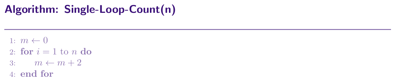
For nested loops, we analyze from inside out, and the total running time is the product of the sizes of all the loops.
for (i = 1; i <= n; i++) {
    for (j = 1; j <= n; j++)
        k = k + 1;   // constant time
}
The inner loop runs exactly $n$ times for each of the $n$ runs of the outer loop. Because this behavior is deterministic and constant across all inputs of size $n$, the tight running time is: \[ c \cdot n \cdot n = \Theta(n^2) \]
When statements come one after another, not nested, we simply add their time complexities.
x = x + 1;   // constant time
for (i = 1; i <= n; i++)
    m = m + 2;   // constant time
for (i = 1; i <= n; i++) {
    for (j = 1; j <= n; j++)
        k = k + 1;   // constant time
}
Total time is: \[ c_0 + c_1 n + c_2 n^2 = \Theta(n^2) \] Here, the largest term, $c_2 n^2$, decides the final order of growth. The smaller terms do not matter for large $n$. Since the execution path always runs both loops, the runtime is tightly bounded by $\Theta(n^2)$.
For an if-else block, the worst-case time is the time for checking the condition, plus the larger of the two branches (the then-part or the else-part).
if (length() == 0)
    return false;      // constant
else {
    for (int n = 0; n < length(); n++) {
        if (list[n].equals(otherList.list[n]))
            return false;   // constant
    }
}
Here, the then part is constant time, but the worst-case scenario for the else part is that the loop runs to completion (taking time proportional to $n$). So, the worst-case complexity is tightly bounded by the else branch:
\[
c_0 + c_1 + (c_2 + c_3)n = \Theta(n)
\]
An algorithm takes $\Theta(\log n)$ time if its problem size gets divided or multiplied by a constant fraction each step, usually by $2$.
for (i = 1; i <= n; i = i * 2)
    ;   // constant time
Here, $i$ doubles every round, so after $k$ rounds, $i = 2^k$. The loop stops precisely when $2^k$ becomes bigger than $n$, which means: \[ 2^k = n \Rightarrow k = \log_2 n \] Since the loop always executes exactly $\lfloor \log_2 n \rfloor + 1$ iterations, its tight bound is $\Theta(\log n)$.
Similarly, dividing by $2$ every round also gives a tight bound of $\Theta(\log n)$:
for (i = n; i >= 1; i = i / 2)
; // constant timeFind the time complexity of this code.
void function(int n) {
    int i, j, k, count = 0;
    for (i = n/2; i <= n; i++)
        for (j = 1; j + n/2 <= n; j++)
            for (k = 1; k <= n; k = k * 2)
                count++;
}
Outer loop: $i$ runs from $n/2$ to $n$, so the number of rounds is exactly $n - n/2 + 1 \approx n/2$, which is $\Theta(n)$.
Middle loop: The condition is $j + n/2 \le n$, which simplifies to $j \le n/2$. So this loop always runs exactly $n/2$ times, which is $\Theta(n)$.
Inner loop: $k$ doubles each round ($1, 2, 4, 8, \dots$) until it exceeds $n$. This always yields exactly $\lfloor \log_2 n \rfloor + 1$ rounds, which is $\Theta(\log n)$.
Combining all three loops: Since these nested loops execute unconditionally, we multiply their tight counts: \[ T(n) = \Theta(n) \times \Theta(n) \times \Theta(\log n) = \Theta(n^2 \log n) \]
Find the time complexity.
for (i = 1; i <= n; i = i + 2)
    count++;
Solution: The loop runs for $i = 1, 3, 5, \dots$, up to $n$, which is exactly $\lceil n/2 \rceil$ rounds. Ignoring the constant factor $\frac{1}{2}$, the tight asymptotic bound is $\Theta(n)$.
Find the time complexity.
for (i = 1; i <= n; i++)
    count++;
for (j = 1; j <= n*n; j++)
    count++;
Solution: The first loop takes exactly $\Theta(n)$ steps and the second loop takes exactly $\Theta(n^2)$ steps. Summing them together, the dominant quadratic term establishes a tight limit, so the total time complexity is $\Theta(n^2)$.
Find the time complexity.
for (i = 1; i <= n; i++)
    for (j = 1; j <= i; j++)
        count++;
Solution: For each $i$, the inner loop runs exactly $i$ times. The total count is: \[ \sum_{i=1}^{n} i = \frac{n(n+1)}{2} \] which is $\Theta(n^2)$.
Find the time complexity.
for (i = 1; i <= n; i++)
    for (j = 1; j <= n; j = j * 2)
        count++;
Solution: The outer loop runs exactly $n$ times ($\Theta(n)$). The inner loop runs exactly $\lfloor \log_2 n \rfloor + 1$ times ($\Theta(\log n)$) for each outer round. Since the work is fully deterministic, the total time complexity is tightly bounded: \[ \Theta(n) \times \Theta(\log n) = \Theta(n \log n) \]
Find the worst-case time complexity.
if (n % 2 == 0) {
    for (i = 1; i <= n; i++)
        count++;
} else {
    for (i = 1; i <= n*n; i++)
        count++;
}
Solution: When $n$ is even, the branch takes exactly $\Theta(n)$ time. When $n$ is odd, the branch takes exactly $\Theta(n^2)$ time. The worst-case performance is strictly determined by the odd branch, meaning the worst-case time complexity is tightly bounded by $\Theta(n^2)$.
This function adds up all numbers from $0$ to $n-1$.
def sum_numbers(n):
    total = 0
    for i in range(n):
        total = total + i   # basic operation
    return total
Analysis: The loop runs exactly $n$ times, and each time, one addition happens. So, \[ C(n) = \sum_{i=0}^{n-1} 1 = n \] This gives $\Theta(n)$.
This function counts how many pairs $(i, j)$ exist, where both $i$ and $j$ range from $0$ to $n-1$.
def count_pairs(n):
    count = 0
    for i in range(n):
        for j in range(n):
            count = count + 1   # basic operation
    return count
Analysis: The outer loop runs $n$ times, and for every round of the outer loop, the inner loop also runs $n$ times. So, \[ C(n) = \sum_{i=0}^{n-1} \sum_{j=0}^{n-1} 1 = n \cdot n = n^2 \] This gives $\Theta(n^2)$.
This function counts pairs $(i, j)$ where $j$ only goes up to $i$, not all the way to $n$.
def count_triangular(n):
    count = 0
    for i in range(n):
        for j in range(i):
            count = count + 1   # basic operation
    return count
Analysis: For a fixed $i$, inner loop runs $i$ times. So, total count is \[ C(n) = \sum_{i=0}^{n-1} i = \frac{n(n-1)}{2} \] This gives $\Theta(n^2)$, the same order as a full nested loop, just with a smaller constant.
This function counts how many times we can double a number, starting from $1$, before it crosses $n$.
def count_doublings(n):
    count = 0
    i = 1
    while i <= n:
        count = count + 1   # basic operation
        i = i * 2
    return count
Analysis: The value of $i$ follows the pattern $1, 2, 4, 8, \dots$, until it crosses $n$. If the loop runs $k$ times, then $2^{k-1} \le n$, so $k \approx \log_2 n$. This gives $\Theta(\log n)$.
This function has a simple loop, followed by a nested loop, one after another, not inside each other.
def mixed_work(n):
    total = 0

    for i in range(n):          # simple loop
        total = total + i

    for i in range(n):          # nested loop
        for j in range(n):
            total = total + 1

    return total
Analysis: The first loop takes $\Theta(n)$ steps. The second, nested loop takes $\Theta(n^2)$ steps. Since these two parts run one after another, we add them together. \[ C(n) = n + n^2 \] For large $n$, the $n^2$ term dominates the $n$ term, so the overall complexity is $\Theta(n^2)$.
Recurrence Relations
A recurrence relation is an equation that defines the running time of an algorithm in terms of its own running time on a smaller input. It is used for recursive algorithms, because a recursive algorithm calls itself on a smaller piece of the problem, and the total time depends on the time of these smaller calls, plus the extra work done outside the calls.
Suppose folding a paper of size $n$ takes some time, and folding always means first folding a paper of half the size, then doing one quick fold action on top. The time to fold size $n$ depends on the time to fold size $n/2$, plus a small constant time for the final fold. This is exactly the idea behind a recurrence relation.
A recurrence relation usually has two parts. One part is the recursive part, which tells the cost in terms of a smaller input. The other part is the base case, which tells the cost when input becomes very small, usually a constant. \[ T(n) = a \cdot T\left(\frac{n}{b}\right) + f(n), T(1) = c \] Here, $a$ is the number of recursive calls made, $\dfrac{n}{b}$ is the size of each smaller call, and $f(n)$ is the extra work done outside the recursive calls, like dividing the problem or combining results.
Merge sort splits an array of size $n$ into two halves, sorts each half recursively, and then merges them. The recurrence relation is \[ T(n) = 2T\left(\frac{n}{2}\right) + cn, T(1) = c \] Here, $2$ recursive calls are made, each on half the size, and $cn$ is the cost of merging.
A recurrence relation only gives the running time indirectly, in terms of itself. To actually know the order of growth, like $\Theta(n \log n)$ or $\Theta(n^2)$, we need to solve the recurrence, that means converting it into a normal formula in terms of $n$ only, without $T$ appearing on the right side.
There are three common methods used to solve a recurrence relation.
Substitution Method, where we guess the answer, and then prove it correct using mathematical induction.
Recursion Tree Method, where we draw the recursive calls as a tree, and add up the work done at every level of the tree.
Master Theorem, which is a ready-made formula, that directly gives the answer for recurrences of a specific common shape.
Substitution Method
In the substitution method, we first guess a formula for $T(n)$, based on intuition or pattern. Then, we substitute this guessed formula back into the recurrence, and check using mathematical induction, whether the guess actually satisfies the recurrence, for all values of $n$.
Step 1: Guess the answer. Based on similar problems, we guess \[ T(n) \le c \cdot n \log n, \text{for some constant } c > 0 \]
Step 2: Assume the guess is true for smaller values. Assume for $n/2$, \[ T\left(\frac{n}{2}\right) \le c \cdot \frac{n}{2} \log\left(\frac{n}{2}\right) \]
Step 3: Substitute into the recurrence. \[ T(n) \le 2 \left( c \cdot \frac{n}{2} \log\left(\frac{n}{2}\right) \right) + n = c \cdot n \log\left(\frac{n}{2}\right) + n \] \[ = c \cdot n (\log n - 1) + n = c \cdot n \log n - c \cdot n + n \]
Step 4: Check the guess. We want \[ c \cdot n \log n - c \cdot n + n \le c \cdot n \log n \] This simplifies to $-c \cdot n + n \le 0$, that means $c \ge 1$. So, choosing $c \ge 1$ works.
Step 5: Conclude. Since a valid $c$ was found, $T(n) = O(n \log n)$. A similar argument with $\ge$ gives $T(n) = \Omega(n \log n)$. So, $T(n) = \Theta(n \log n)$.
Step 1: Guess the answer. We guess \[ T(n) \le c \cdot \log n, \text{for some constant } c > 0 \]
Step 2: Assume the guess is true for $n/2$. \[ T\left(\frac{n}{2}\right) \le c \cdot \log\left(\frac{n}{2}\right) \]
Step 3: Substitute into the recurrence. \[ T(n) \le c \cdot \log\left(\frac{n}{2}\right) + 1 = c (\log n - 1) + 1 = c \log n - c + 1 \]
Step 4: Check the guess. We want \[ c \log n - c + 1 \le c \log n \] This simplifies to $-c + 1 \le 0$, that means $c \ge 1$. So, choosing $c \ge 1$ works.
Step 5: Conclude. So, $T(n) = O(\log n)$. A similar argument gives $T(n) = \Omega(\log n)$. So, $T(n) = \Theta(\log n)$.
Step 1: Guess the answer. We guess \[ T(n) \le c \cdot n^2, \text{for some constant } c > 0 \]
Step 2: Assume the guess is true for $n/2$. \[ T\left(\frac{n}{2}\right) \le c \cdot \left(\frac{n}{2}\right)^2 = c \cdot \frac{n^2}{4} \]
Step 3: Substitute into the recurrence. \[ T(n) \le 2 \left( c \cdot \frac{n^2}{4} \right) + n^2 = \frac{c \cdot n^2}{2} + n^2 \]
Step 4: Check the guess. We want \[ \frac{c \cdot n^2}{2} + n^2 \le c \cdot n^2 \] This simplifies to $n^2 \le \dfrac{c \cdot n^2}{2}$, that means $c \ge 2$. So, choosing $c \ge 2$ works.
Step 5: Conclude. So, $T(n) = O(n^2)$. A similar argument gives $T(n) = \Omega(n^2)$. So, $T(n) = \Theta(n^2)$.
Recursion Tree Method
In the recursion tree method, we draw a tree, where the root is the original problem of size $n$, and the children of each node are the smaller recursive calls made by that node. Each node also carries the extra cost $f(n)$ done at that level, not counting its children's cost. We then add up the cost of every level, and add all levels together, to get the total cost.
Step 1: Draw the root. The root is a problem of size $n$, with cost $n$ at that level.
Step 2: Draw the children. The root makes $2$ calls of size $n/2$ each. Level cost is $2 \times \dfrac{n}{2} = n$.
Step 3: Continue expanding. Each of those $2$ nodes makes $2$ calls of size $n/4$. Now $4$ nodes exist, each cost $n/4$, level total $4 \times \dfrac{n}{4} = n$.
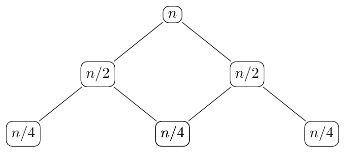
Step 4: Notice the pattern. Every level costs exactly $n$, since problem size halves but number of nodes doubles, and these effects cancel.
Step 5: Count the levels. Size goes $n, n/2, n/4, \dots, 1$, giving $\log_2 n$ levels.
Step 6: Total cost. \[ T(n) = n \times \log_2 n = \Theta(n \log n) \]
Step 1: Draw the root. Root is size $n$, cost $n$.
Step 2: Draw children. Root makes $3$ calls of size $n/2$. Level cost $3 \times \dfrac{n}{2} = \dfrac{3n}{2}$.
Step 3: Continue expanding. Each of those $3$ nodes makes $3$ calls of size $n/4$, giving $9$ nodes, level cost $9 \times \dfrac{n}{4} = \dfrac{9n}{4}$.
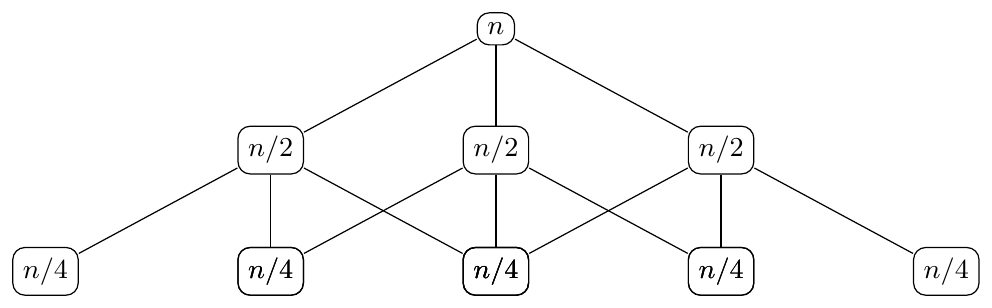
Step 4: Notice the pattern. At level $i$, there are $3^i$ nodes, each of size $n/2^i$, so level cost is $3^i \times \dfrac{n}{2^i} = n \left(\dfrac{3}{2}\right)^i$. This level cost increases as $i$ increases, since $3/2 > 1$.
Step 5: Count the levels. Number of levels is $\log_2 n$, since size halves every level.
Step 6: Total cost. Since the cost grows with each level, the last level dominates the sum. The last level has $n^{\log_2 3}$ nodes, each doing constant work, giving \[ T(n) = \Theta(n^{\log_2 3}) \] which is approximately $\Theta(n^{1.58})$.
Step 1: Draw the root. Root is size $n$, cost $n$.
Step 2: Draw children. Root makes $2$ calls, one of size $n/2$, one of size $n/4$. Level cost is $\dfrac{n}{2} + \dfrac{n}{4} = \dfrac{3n}{4}$.
Step 3: Continue expanding. The $n/2$ node makes calls of size $n/4$ and $n/8$. The $n/4$ node makes calls of size $n/8$ and $n/16$. Level cost is again less than $n$, around $\dfrac{9n}{16}$.
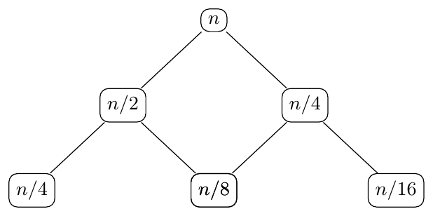
Step 4: Notice the pattern. Unlike Example 2, here the level cost keeps shrinking, since $\dfrac{1}{2} + \dfrac{1}{4} = \dfrac{3}{4} < 1$. So the root level cost, $n$, dominates the total sum.
Step 5: Total cost. Adding up a shrinking sum across all levels still gives a value close to the root cost, just scaled by a constant. So, \[ T(n) = \Theta(n) \]
Extended Master Theorem
The Extended Master Theorem solves recurrences of the form \[ T(n) = a \cdot T\left(\frac{n}{b}\right) + \Theta(n^k \log^p n) \] where $a \ge 1$, $b > 1$, $k \ge 0$ are constants, and $p$ is any real number. Instead of comparing $f(n)$ with $n^{\log_b a}$ directly, we identify the constants $a$, $b$, $k$, $p$, then compare $a$ with $b^k$.
Case 1: If $a > b^k$, the work done by the leaves dominates, then \[ T(n) = \Theta(n^{\log_b a}) \]
Case 2: If $a = b^k$, the work is balanced across all levels, and the log power $p$ decides the answer:
\[
T(n) = \begin{cases}
\Theta(n^{\log_b a} \log^{p+1} n) & p > -1
\Theta(n^{\log_b a} \log \log n) & p = -1
\Theta(n^{\log_b a}) & p < -1
\end{cases}
\]
Case 3: If $a < b^k$, the work done at the root dominates, and $p$ decides the answer:
\[
T(n) = \begin{cases}
\Theta(n^k \log^p n) & p \ge 0
\Theta(n^k) & p < 0
\end{cases}
\]
Step 1: Identify constants. $a = 2$, $b = 2$, $f(n) = n = \Theta(n^1 \log^0 n)$, so $k = 1$, $p = 0$.
Step 2: Compare $a$ with $b^k$. \[ a = 2, b^k = 2^1 = 2 \Rightarrow a = b^k \]
Step 3: Apply Case 2, check $p$. Since $p = 0 > -1$, use the first sub-case.
Step 4: Compute the answer. \[ T(n) = \Theta(n^{\log_2 2} \log^{0+1} n) = \Theta(n \log n) \]
Step 1: Identify constants. $a = 9$, $b = 3$, $f(n) = n = \Theta(n^1 \log^0 n)$, so $k = 1$, $p = 0$.
Step 2: Compare $a$ with $b^k$. \[ a = 9, b^k = 3^1 = 3 \Rightarrow a > b^k \]
Step 3: Apply Case 1. The leaves dominate since $a > b^k$.
Step 4: Compute the answer. \[ T(n) = \Theta(n^{\log_3 9}) = \Theta(n^2) \]
Step 1: Identify constants. $a = 3$, $b = 4$, $f(n) = n\log n = \Theta(n^1 \log^1 n)$, so $k = 1$, $p = 1$.
Step 2: Compare $a$ with $b^k$. \[ a = 3, b^k = 4^1 = 4 \Rightarrow a < b^k \]
Step 3: Apply Case 3, check $p$. Since $p = 1 \ge 0$, use the first sub-case.
Step 4: Compute the answer. \[ T(n) = \Theta(n^k \log^p n) = \Theta(n \log n) \]
The Extended Master Theorem still fails to apply when the recurrence does not fit the exact form $a \cdot T(n/b) + \Theta(n^k \log^p n)$. This happens when $a < 1$, since that is not a valid divide-and-conquer split, or when the subproblem sizes are unequal, like $T(n) = T(n/2) + T(n/3) + n$, or when $f(n)$ is not of the form $n^k \log^p n$ at all, for example $f(n) = 2^n$. In such cases, we go back to the recursion tree method or the Akra-Bazzi method.
Step 1: Identify constants. $a = 2$, $b = 2$, $f(n) = n \log n = \Theta(n^1 \log^1 n)$, so $k = 1$, $p = 1$.
Step 2: Compare $a$ with $b^k$. \[ a = 2, b^k = 2^1 = 2 \Rightarrow a = b^k \]
Step 3: Apply Case 2, check $p$. Since $p = 1 > -1$, use the first sub-case.
Step 4: Compute the answer. \[ T(n) = \Theta(n^{\log_2 2} \log^{1+1} n) = \Theta(n \log^2 n) \] This is exactly the recurrence that the basic Master Theorem could not solve, since $f(n) = n \log n$ sits exactly on $n^{\log_b a} = n$ with an extra log factor. The extended version handles it directly through the $p$ sub-case.
Solve $T(n) = 4T(n/2) + n$ using the Extended Master Theorem.
Solution: $a = 4$, $b = 2$, $f(n) = n = \Theta(n^1 \log^0 n)$, so $k = 1$, $p = 0$. $b^k = 2^1 = 2$. Since $a = 4 > b^k = 2$, this is Case 1, giving $T(n) = \Theta(n^{\log_2 4}) = \Theta(n^2)$.
Solve $T(n) = 2T(n/2) + n^2$ using the Extended Master Theorem.
Solution: $a = 2$, $b = 2$, $f(n) = n^2 = \Theta(n^2 \log^0 n)$, so $k = 2$, $p = 0$. $b^k = 2^2 = 4$. Since $a = 2 < b^k = 4$, this is Case 3, and $p = 0 \ge 0$, giving $T(n) = \Theta(n^2 \log^0 n) = \Theta(n^2)$.
Solve $T(n) = 8T(n/2) + n^2$ using the Extended Master Theorem.
Solution: $a = 8$, $b = 2$, $f(n) = n^2 = \Theta(n^2 \log^0 n)$, so $k = 2$, $p = 0$. $b^k = 2^2 = 4$. Since $a = 8 > b^k = 4$, this is Case 1, giving $T(n) = \Theta(n^{\log_2 8}) = \Theta(n^3)$.
Solve $T(n) = T(n/2) + n$ using the Extended Master Theorem.
Solution: $a = 1$, $b = 2$, $f(n) = n = \Theta(n^1 \log^0 n)$, so $k = 1$, $p = 0$. $b^k = 2^1 = 2$. Since $a = 1 < b^k = 2$, this is Case 3, and $p = 0 \ge 0$, giving $T(n) = \Theta(n^1 \log^0 n) = \Theta(n)$.
Solve $T(n) = 4T(n/2) + n \log^{-1} n$ using the Extended Master Theorem.
Solution: $a = 4$, $b = 2$, $f(n) = n\log^{-1} n = \Theta(n^1 \log^{-1} n)$, so $k = 1$, $p = -1$. $b^k = 2^1 = 2$. Since $a = 4 > b^k = 2$, this is Case 1, and Case 1 does not depend on $p$ at all, giving $T(n) = \Theta(n^{\log_2 4}) = \Theta(n^2)$.
Analysis of Recursive Algorithms
A recursive algorithm is an algorithm that calls itself on a smaller input, until it reaches a base case, which is the simplest input that needs no further recursion. To analyze a recursive algorithm, we first write its recurrence relation, by checking how many recursive calls happen, how much smaller the input becomes, and how much extra work happens outside the calls. Then, we solve this recurrence using substitution, recursion tree, or master theorem, to get the final order of growth.
Decide the input size parameter, usually $n$.
Identify the basic operation, the operation that repeats with every call.
Find how many recursive calls are made, and on what smaller size.
Write the recurrence relation, including the base case.
Solve the recurrence to get the order of growth.
Factorial Function
Factorial of $n$, written $n!$, means multiplying all numbers from $n$ down to $1$. The recursive idea is, $n! = n \times (n-1)!$, and the base case is $0! = 1$. So, computing factorial of $n$ depends on computing factorial of $n-1$ first.
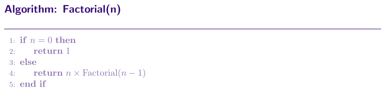
Factorial(n)
if n == 0
return 1
else
return n * Factorial(n - 1)
def factorial(n):
    if n == 0:
        return 1
    else:
return n * factorial(n - 1)Step 1: Input size. The parameter $n$ is the input size.
Step 2: Basic operation. The multiplication, $n \times \text{Factorial}(n-1)$, is the basic operation.
Step 3: Recursive calls. Each call makes exactly $1$ recursive call, on input size $n-1$.
Step 4: Recurrence relation. \[ T(n) = T(n-1) + c, T(0) = c \] Here, $c$ represents the constant work done outside the recursive call, like the multiplication and the comparison.
Step 5: Solve. Using the recursion tree method, each level reduces $n$ by $1$, and does constant work $c$. The tree has $n+1$ levels, from $n$ down to $0$. Total cost is \[ T(n) = c \times (n+1) = \Theta(n) \]
Fibonacci Function
The Fibonacci sequence is $0, 1, 1, 2, 3, 5, 8, \dots$, where each number is the sum of the two numbers before it. The recursive idea is, $\text{Fib}(n) = \text{Fib}(n-1) + \text{Fib}(n-2)$, with base cases $\text{Fib}(0) = 0$ and $\text{Fib}(1) = 1$. Unlike factorial, here each call makes two recursive calls, not one.
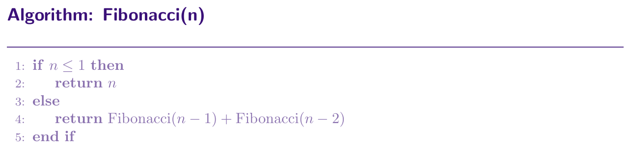
Fibonacci(n)
if n $<=$ 1
return n
else
return Fibonacci(n - 1) + Fibonacci(n - 2)
def fibonacci(n):
    if n <= 1:
        return n
    else:
return fibonacci(n - 1) + fibonacci(n - 2)Step 1: Input size. The parameter $n$ is the input size.
Step 2: Basic operation. The addition, combining the two recursive results, is the basic operation.
Step 3: Recursive calls. Each call makes $2$ recursive calls, one on $n-1$, one on $n-2$.
Step 4: Recurrence relation. \[ T(n) = T(n-1) + T(n-2) + c, T(0) = T(1) = c \]
Step 5: Solve. This recurrence does not fit the Master Theorem, since the two subproblems have different sizes. Using the recursion tree method, each call branches into $2$ more calls, so the tree looks similar to a binary tree, except the depth on the left branch is longer than the right branch. The total number of nodes in this tree can be shown to grow like the Fibonacci numbers themselves, giving \[ T(n) = \Theta(\phi^n), \phi \approx 1.618 \] where $\phi$ is the golden ratio. So, this simple looking function has exponential running time, $\Theta(2^n)$ is also commonly used as a simpler, looser bound for this.
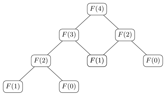
The picture shows the recursion tree for $\text{Fib}(4)$. Notice that $F(2)$ and $F(1)$ are computed many times, again and again, which is the reason this recursion is so slow.
Sum of Digits Function
This function adds up all the digits of a number $n$. The recursive idea is, the sum of digits of $n$ equals the last digit of $n$, plus the sum of digits of the remaining number, after removing the last digit. The base case is, when $n$ becomes $0$, the sum is $0$.
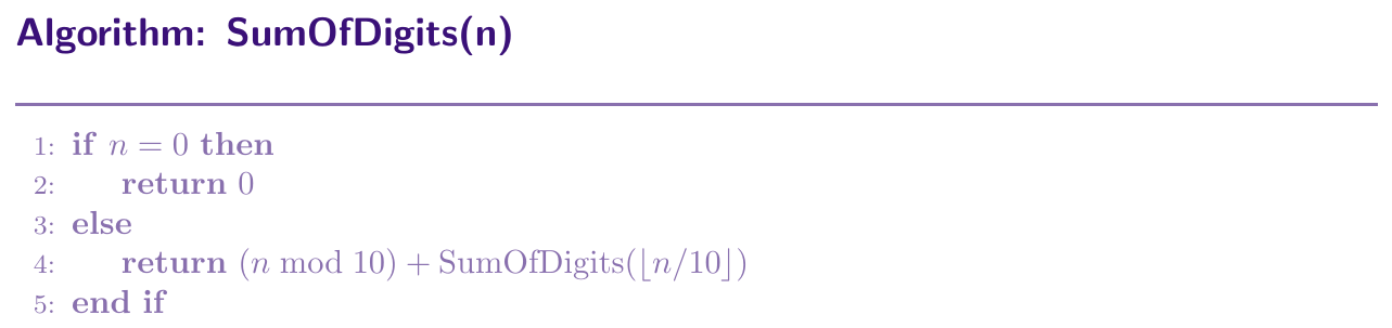
SumOfDigits(n)
if n == 0
return 0
else
return (n mod 10) + SumOfDigits(n / 10)
def sum_of_digits(n):
    if n == 0:
        return 0
    else:
return (n % 10) + sum_of_digits(n // 10)Step 1: Input size. Here, the input size is not $n$ itself, but the number of digits in $n$, since each call removes one digit, not one unit. Let us call the number of digits $d$.
Step 2: Basic operation. The addition, $(n \bmod 10) + \text{SumOfDigits}(n/10)$, is the basic operation.
Step 3: Recursive calls. Each call makes exactly $1$ recursive call, on a number with one less digit.
Step 4: Recurrence relation. \[ T(d) = T(d-1) + c, T(0) = c \]
Step 5: Solve. Same pattern as factorial, each level does constant work, and there are $d+1$ levels. Total cost is \[ T(d) = \Theta(d) \] Since $d \approx \log_{10} n$, we can also write this as $\Theta(\log n)$, in terms of the value of $n$.
Power Function
This function computes $x^n$, that is $x$ raised to power $n$. There are two ways to write this recursively, a slow way and a fast way. We look at both, to see how the recurrence changes the running time.
Here, $x^n = x \times x^{n-1}$, with base case $x^0 = 1$.
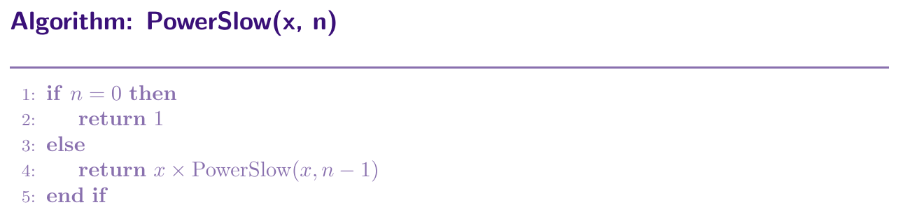
def power_slow(x, n):
    if n == 0:
        return 1
    else:
        return x * power_slow(x, n - 1)
Recurrence: $T(n) = T(n-1) + c$, giving $T(n) = \Theta(n)$, same pattern as factorial.
Here, we use the idea, $x^n = (x^{n/2})^2$, when $n$ is even, and $x^n = x \times (x^{(n-1)/2})^2$, when $n$ is odd. This way, the power reduces to half each time, instead of reducing by $1$.
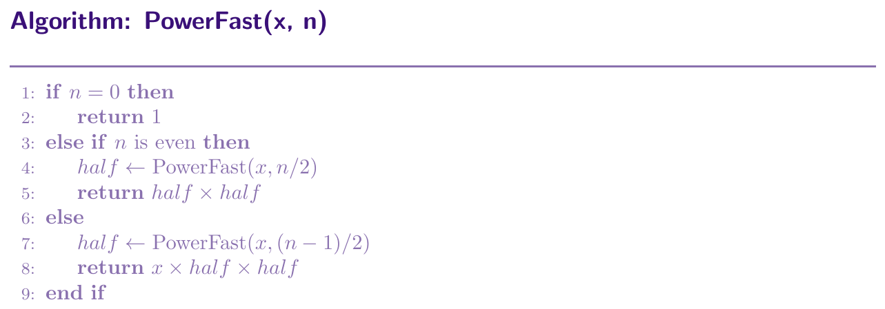
PowerFast(x, n)
if n == 0
return 1
else if n is even
half = PowerFast(x, n / 2)
return half * half
else
half = PowerFast(x, (n - 1) / 2)
return x * half * half
def power_fast(x, n):
    if n == 0:
        return 1
    elif n % 2 == 0:
        half = power_fast(x, n // 2)
        return half * half
    else:
        half = power_fast(x, (n - 1) // 2)
return x * half * halfStep 1: Input size. The parameter $n$ is the input size.
Step 2: Basic operation. The multiplication, $half \times half$, is the basic operation.
Step 3: Recursive calls. Each call makes exactly $1$ recursive call, on input size roughly $n/2$.
Step 4: Recurrence relation. \[ T(n) = T(n/2) + c, T(0) = c \]
Step 5: Solve using Master Theorem. Here, $a = 1$, $b = 2$, $f(n) = c = \Theta(1) = \Theta(n^0)$. Compute $n^{\log_b a} = n^{\log_2 1} = n^0$. Since $f(n)$ matches $n^{\log_b a}$ exactly, this is Case 2, giving \[ T(n) = \Theta(n^0 \log n) = \Theta(\log n) \] This shows the fast version is much better than the slow version, $\Theta(\log n)$ compared to $\Theta(n)$, just by halving the power instead of reducing it by $1$ each time.
A function reverses the digits of a number $n$ recursively, removing one digit and placing it at the end, in each call, until $n$ becomes $0$. Identify the recurrence and find the order of growth.
Solution: Each call reduces the number of digits by $1$, doing constant work. So, $T(d) = T(d-1) + c$, giving $T(d) = \Theta(d) = \Theta(\log n)$.
A function adds up all elements of an array of size $n$, by adding the first element to the sum of the rest of the array, recursively. Identify the recurrence and find the order of growth.
Solution: Each call reduces array size by $1$, doing constant work to add one element. So, $T(n) = T(n-1) + c$, giving $T(n) = \Theta(n)$.
The Tower of Hanoi problem moves $n$ disks, by first moving $n-1$ disks to a spare rod, then moving the largest disk, then moving the $n-1$ disks again, on top of it. Identify the recurrence and find the order of growth.
Solution: Each call makes $2$ recursive calls, each on size $n-1$, plus constant work for moving the largest disk. So, $T(n) = 2T(n-1) + c$. Solving by recursion tree, the tree doubles in nodes each level, while the work per node stays constant, giving $T(n) = \Theta(2^n)$.
A function prints numbers from $n$ down to $1$, by printing $n$, then calling itself on $n-1$. Identify the recurrence and find the order of growth.
Solution: Each call reduces $n$ by $1$, doing constant work for the print statement. So, $T(n) = T(n-1) + c$, giving $T(n) = \Theta(n)$.
A function computes the GCD of two numbers $a$ and $b$, using $\text{GCD}(a, b) = \text{GCD}(b, a \bmod b)$, until $b$ becomes $0$. This problem is harder to analyze directly using $n$ as size, since the reduction is not a simple halving or minus one, it depends on number theory properties.
Solution: It is known, using a deeper number theory result, that this recursion takes at most $O(\log(\min(a,b)))$ calls, because the smaller number reduces roughly by a multiplicative factor related to the golden ratio, in the worst case, every two calls.
Useful Formulas
A. Core Logarithm Identities
(All logarithms below are base $2$ unless stated otherwise; the base never affects $\Theta$-notation.)
Product rule: $\log(mn) = \log m + \log n$
Example: $\log(8n) = 3 + \log n$.Quotient rule: $\log(m/n) = \log m - \log n$
Example: $\log(n/4) = \log n - 2$.Power rule: $\log(n^k) = k \log n$
Example: $\log(n^3) = 3 \log n$.Change of base: $\log_b n = \dfrac{\log_a n}{\log_a b}$
Example: $\log_2 n = \dfrac{\ln n}{\ln 2}$, so $\log_2 n = \Theta(\ln n)$ – this is exactly why the base of a log is never written inside $\Theta$-notation: changing the base only multiplies by a constant.Inverse identity: $b^{\log_b n} = n$
Example: $2^{\log_2 n} = n$.Base facts: $\log_b 1 = 0$, $\log_b b = 1$.
Exponent–log swap (the “hidden” identity): $a^{\log_b c} = c^{\log_b a}$
Example: $n^{\log_2 7} = 7^{\log_2 n}$ – this rewriting is exactly how divide-and-conquer exponents like $\Theta(n^{\log_2 7})$ are manipulated.The “$n^{1/\log n}$ is a constant” trick: $n^{1/\log_b n} = b$
Example: $n^{1/\log_2 n} = 2$ for every $n$ – a function that looks like it depends on $n$ but is actually $\Theta(1)$.Sum of logs $=$ log of a factorial: $\displaystyle\sum_{i=1}^{n} \log i = \log(n!)$
Example: this identity is the bridge to Stirling's Approximation in Section B below.For very small x, $\log_{b}(1+x) \approx \frac{x}{\ln(b)}$, where $ln$ is natural logarithm ( base e).
Iterated logarithm $\log^{*} n$: the number of times $\log$ must be applied to $n$ before the result is $\le 1$. It grows slower than $\log\log\cdots\log n$ for any fixed number of iterations.
Example: $\log^{*}(65536) = 4$, since $\log\log\log\log(65536) \le 1$; for all practically occurring $n$, $\log^{*} n \le 5$.
B. Factorial and Stirling's Approximation
Stirling's Approximation: \[n! = \sqrt{2\pi n}\left(\frac{n}{e}\right)^n\left(1 + O\!\left(\frac{1}{n}\right)\right) \Longrightarrow n! = \Theta\!\left(\sqrt{n}\left(\frac{n}{e}\right)^n\right)\] Example: for $n=10$, Stirling gives $10! \approx 3{,}598{,}696$, versus the true value $3{,}628{,}800$ – accurate to within $1\%$.
Log-factorial form (the single most-used consequence of Stirling): \[\ln(n!) = n\ln n - n + O(\log n) \Longrightarrow \log(n!) = \Theta(n \log n)\] Example: this is precisely why the comparison-based sorting lower bound is $\Omega(n \log n)$, and why $\log(n!)$ and $n \log n$ can always be swapped inside $\Theta$-notation.
Loose factorial bounds (no constants needed): \[\left(\frac{n}{e}\right)^n \;\le\; n! \;\le\; n^n\] Example: instantly bounds $n!$ between an exponential and $n^n$ without invoking $\sqrt{2\pi n}$.
Factorial's place in the growth hierarchy: for every constant $c$, \[c^n = o(n!) \text{and} n! = o(n^n)\] Example: $2^n = o(n!)$ and $n! = o(n^n)$, so $2^n \prec n! \prec n^n$.
Central binomial coefficient: \[\binom{2n}{n} \sim \frac{4^n}{\sqrt{\pi n}} \Longrightarrow \binom{2n}{n} = \Theta\!\left(\frac{4^n}{\sqrt n}\right)\] Example: shows $\binom{2n}{n} = O(4^n)$ but $\binom{2n}{n} \ne \Theta(4^n)$ – the $\sqrt n$ factor in the denominator matters.
Sum of all binomial coefficients: \[\sum_{k=0}^{n} \binom{n}{k} = 2^n\] Example: this is exactly the count of all $2^n$ subsets of an $n$-element set – the standard justification for a Brute-Force paradigm's exponential running time.
C. Summation (Series) Formulas
Arithmetic series: \[\sum_{i=1}^{n} i = \frac{n(n+1)}{2} = \Theta(n^2)\]
Sum of squares: \[\sum_{i=1}^{n} i^2 = \frac{n(n+1)(2n+1)}{6} = \Theta(n^3)\]
Sum of cubes: \[\sum_{i=1}^{n} i^3 = \left(\frac{n(n+1)}{2}\right)^2 = \Theta(n^4)\]
General power sum: \[\sum_{i=1}^{n} i^k = \Theta(n^{k+1}), \text{for any constant } k \ge 0\]
Finite geometric series
For $r > 1$: $S_n = \frac{a(r^n - 1)}{r - 1}$
For $r < 1$: $S_n = \frac{a(1 - r^n)}{1 - r}$
For $S_\infty$ ($|r| < 1$): $S_\infty = \frac{a}{1 - r}$
Harmonic series: \[\sum_{i=1}^{n} \frac{1}{i} = \ln n + \gamma + O(1/n) = \Theta(\log n), \gamma \approx 0.5772\] Example: directly explains why a loop of the form
for(i=1;i<=n;i++) for(j=1;j<=n;j+=i)runs $\Theta(n \log n)$ times in total.Sum of logarithms: \[\sum_{i=1}^{n} \log i = \log(n!) = \Theta(n \log n)\]
Arithmetico-geometric series ($r > 1$): \[\sum_{i=1}^{n} i \, r^i = \Theta(n \, r^n)\] Example: $\displaystyle\sum_{i=1}^{n} i \cdot 2^i = \Theta(n \cdot 2^n)$ – again dominated by the last (largest-index) term.
Decaying recursion-tree workload: \[\sum_{i=0}^{\log n} \frac{n}{2^i} = \Theta(n)\] Example: models a divide-and-conquer process where the work per level halves but the number of levels is $\Theta(\log n)$ – the total is still only $\Theta(n)$, not $\Theta(n \log n)$.
Growing recursion-tree workload: \[\sum_{i=1}^{\log n} 2^i = \Theta(n)\] Example: work doubling every level for $\Theta(\log n)$ levels also sums to only $\Theta(n)$, since the sum is dominated by the final, largest term.
D. Growth-Rate Hierarchy and Limit Tests
Logarithms lose to every polynomial: \[\lim_{n \to \infty} \frac{\log n}{n^{\varepsilon}} = 0, \text{for any constant } \varepsilon > 0\] Example: $\log n = o(\sqrt n)$, and even $\log n = o(n^{0.001})$.
Polynomials lose to every exponential: \[\lim_{n \to \infty} \frac{n^{k}}{c^{n}} = 0, \text{for any constants } k > 0,\ c > 1\] Example: $n^{100} = o(1.01^n)$.
The full growth hierarchy (for constants $0<\varepsilon<1$ and $c>1$): \[\log^{*} n \;\prec\; \log\log n \;\prec\; \log n \;\prec\; n^{\varepsilon} \;\prec\; n \;\prec\; n\log n \;\prec\; n^{c} \;\prec\; c^{n} \;\prec\; n! \;\prec\; n^{n}\]
Ratio (limit) test for comparing $f$ and $g$: if $\displaystyle\lim_{n\to\infty}\frac{f(n)}{g(n)} = L$, then \[0 < L < \infty \Rightarrow f = \Theta(g), L = 0 \Rightarrow f = o(g), L = \infty \Rightarrow f = \omega(g)\] Example: $\displaystyle\lim_{n\to\infty} \frac{3n^2+5}{n^2} = 3 \Rightarrow 3n^2+5 = \Theta(n^2)$.
Euler's number limits (used in hashing / amortized / probabilistic analyses): \[\lim_{n\to\infty}\left(1+\frac{1}{n}\right)^{n} = e, \lim_{n\to\infty}\left(1-\frac{1}{n}\right)^{n} = \frac{1}{e}\] Example: the probability that $n$ items hashed into $n$ buckets avoid a particular bucket entirely is $(1-1/n)^n \approx 1/e$.
Exponential and log inequalities (used to bound the expressions above): \[1 + x \le e^{x} \ \text{ for all real } x, \ln(1+x) \le x \ \text{ for } x > -1\] Example: gives the one-line bound $(1 - 1/n)^n \le e^{-1}$ used just above.
E. Floors/ceilings never matter
For a recurrence $T(n) = a\,T(n/b) + f(n)$ with $a \ge 1$, $b > 1$, let $p = \log_b a$.
Floors/ceilings never matter: $T(n) = T(\lfloor n/2 \rfloor) + T(\lceil n/2 \rceil) + O(n)$ has exactly the same solution, $\Theta(n\log n)$, as $T(n) = 2T(n/2) + O(n)$.