Hash Tables
Hash Functions and Load Factor
A hash function $h(k)$ takes a key $k$ and maps it to an integer in the range $[0, m-1]$, where $m$ is the size of the hash table array. A good hash function should:
Be fast to compute.
Distribute keys uniformly across the array, to avoid many keys landing at the same position.
Be deterministic, meaning the same key always gives the same index.
Division Method
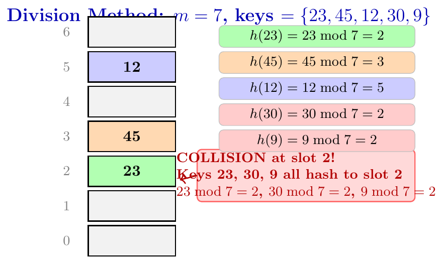
The simplest hash function. We divide the key by the table size $m$ and take the remainder. \[ h(k) = k \bmod m \] For example, if $m = 7$ and key $k = 23$, then $h(23) = 23 \bmod 7 = 2$. Key 23 goes to slot 2.
Choosing $m$: A prime number that is not close to a power of 2 works best for $m$. For example, if we have 1000 entries, choosing $m = 997$ (a prime) distributes better than $m = 1024 = 2^{10}$.
Table size $m = 7$. Insert keys: $\{23, 45, 12, 30, 9\}$.
$h(23) = 23 \bmod 7 = 2 \to$ slot 2
$h(45) = 45 \bmod 7 = 3 \to$ slot 3
$h(12) = 12 \bmod 7 = 5 \to$ slot 5
$h(30) = 30 \bmod 7 = 2 \to$ slot 2 (COLLISION with 23!)
$h(9) = 9 \bmod 7 = 2 \to$ slot 2 (COLLISION again!)
Multiplication Method
In the multiplication method, we multiply the key by a constant $A$ (where $0 < A < 1$), take the fractional part of the result, and then multiply by $m$. \[ h(k) = \lfloor m \cdot (k \cdot A \bmod 1) \rfloor \] Here, $k \cdot A \bmod 1$ means we take only the fractional part of $k \cdot A$. A commonly used value is $A = \dfrac{\sqrt{5}-1}{2} \approx 0.6180$, known as the golden ratio conjugate. This method works for any value of $m$, and powers of 2 are fine for $m$ here.
Let $m = 8$, $A = 0.6180$, key $k = 23$.
$k \cdot A = 23 \times 0.6180 = 14.214$
Fractional part $= 0.214$
$h(23) = \lfloor 8 \times 0.214 \rfloor = \lfloor 1.712 \rfloor = 1$
So key 23 goes to slot 1.
Load Factor
The load factor $\alpha$ tells us how full the hash table is. \[ \alpha = \frac{n}{m} \] where $n$ is the number of keys currently stored in the table, and $m$ is the total number of slots. The load factor directly affects performance.
When $\alpha$ is small (table mostly empty), collisions are rare, and operations are fast.
When $\alpha$ is large (table mostly full), collisions are frequent, and operations become slow.
For chaining, $\alpha$ can be $> 1$ (more keys than slots).
For open addressing, $\alpha$ must be $< 1$ (we need at least one empty slot).
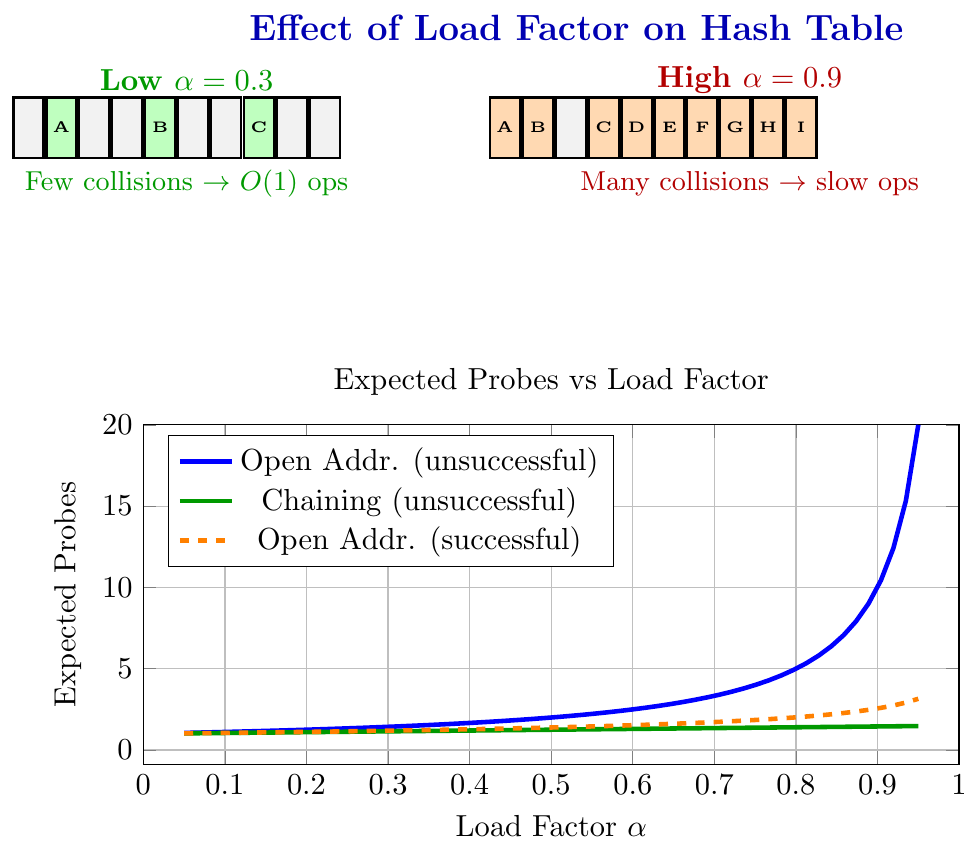
Suppose table size $m = 10$ and we insert $n = 7$ keys. Then $\alpha = 7/10 = 0.7$. This means 70\% of slots are occupied. The remaining 30\% are empty. Each new insertion is likely to find a collision, taking more time to find an empty slot. If we had $m = 20$ for the same 7 keys, $\alpha = 0.35$, and performance would be much better.
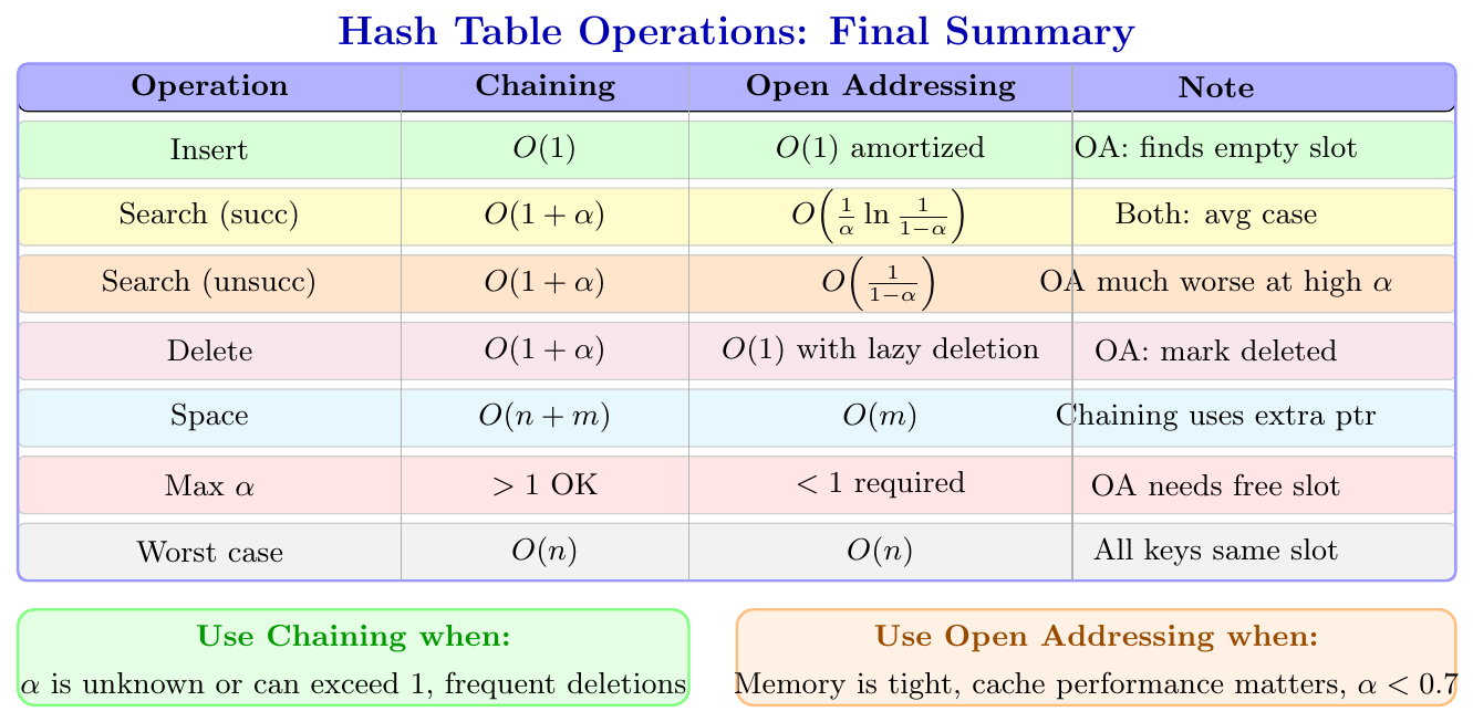
Under the assumption of simple uniform hashing (each key is equally likely to hash to any slot, independently), the expected time for insert, search, and delete is $O(1)$ when the load factor $\alpha$ is kept constant. This is why hash tables are called $O(1)$ data structures in practice. However, in the worst case (all $n$ keys hash to the same slot), operations take $O(n)$.
Collision Resolution
A collision happens when two different keys $k_1$ and $k_2$ produce the same hash value, meaning $h(k_1) = h(k_2)$. Since there are infinitely many possible keys but only $m$ slots, collisions are unavoidable (Pigeonhole Principle). We must handle them. There are two main strategies: Chaining and Open Addressing.
Chaining (Separate Chaining)
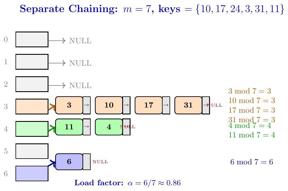
In chaining, each slot of the hash table holds a linked list (or chain) of all keys that hash to that slot. When a collision occurs, we simply add the new key to the linked list at that slot. There is no limit on how many keys can go into the same slot.
Insert: Hash the key, go to that slot, add the key to the front of the linked list. $O(1)$.
Search: Hash the key, go to that slot, search the linked list at that slot. Average $O(1+\alpha)$.
Delete: Hash the key, go to that slot, find and remove from the linked list. Average $O(1+\alpha)$.
Table size $m = 5$. Insert keys: $\{12, 17, 22, 3, 7, 27\}$ using $h(k) = k \bmod 5$.
$h(12) = 2 \to$ slot 2: [12]
$h(17) = 2 \to$ slot 2: [17, 12] (collision, added to chain)
$h(22) = 2 \to$ slot 2: [22, 17, 12] (another collision)
$h(3) = 3 \to$ slot 3: [3]
$h(7) = 2 \to$ slot 2: [7, 22, 17, 12]
$h(27) = 2 \to$ slot 2: [27, 7, 22, 17, 12]
Here, $\alpha = 6/5 = 1.2 > 1$ (allowed in chaining!). Slot 2 has a very long chain, which is bad.
class ChainingHashTable:
    def __init__(self, m):
        self.m    = m
        self.table = [[] for _ in range(m)]  # each slot is a list

    def hash(self, key):
        return key % self.m              # division method

    def insert(self, key):
        slot = self.hash(key)
        if key not in self.table[slot]:  # avoid duplicates
            self.table[slot].insert(0, key)  # insert at front O(1)

    def search(self, key):
        slot = self.hash(key)
        return key in self.table[slot]   # search the chain

    def delete(self, key):
        slot = self.hash(key)
        if key in self.table[slot]:
            self.table[slot].remove(key)
        else:
            print(f"{key} not found")

    def display(self):
        for i, chain in enumerate(self.table):
            print(f"Slot {i}: {chain}")


# --- Driver Code ---
ht = ChainingHashTable(7)
for key in [10, 20, 15, 7, 3, 24]:
    ht.insert(key)
ht.display()
# Slot 0: [7]
# Slot 1: [15]
# Slot 2: [2]
# Slot 3: [10, 3]
# Slot 4: []
# Slot 5: []
# Slot 6: [20]
print("Search 10:", ht.search(10))   # True
ht.delete(10)
print("Search 10:", ht.search(10))   # False
Open Addressing
In open addressing, all keys are stored directly in the hash table array itself. There are no linked lists. If a collision occurs at slot $h(k)$, we probe other slots in a specific sequence until we find an empty slot. The probing sequence is determined by a probe function $h(k, i)$, where $i$ is the probe number (0, 1, 2, \ldots). We always have $\alpha < 1$ because every key needs its own slot.
The key rule: When searching for a key, we follow the same probe sequence. When we find an empty slot, we stop (key not present). When we find the key, we stop (found).
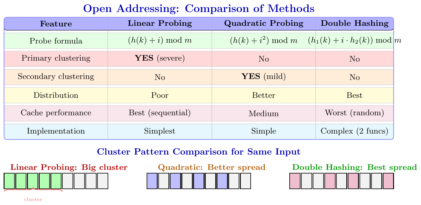
Linear Probing
In linear probing, when a collision occurs at slot $h(k)$, we simply move to the next slot, and then the next, and so on, one step at a time. \[ h(k, i) = (h(k) + i) \bmod m, i = 0, 1, 2, \ldots \] So if $h(k) = 3$ and slot 3 is occupied, we try slot 4, then 5, then 6, and so on, wrapping around if needed.
Analogy: Think of looking for a parking spot in a lot. You drove to your preferred spot (your hash slot). It is taken. So you look at the next spot, then the next, going one by one until you find a free one.
Table size $m = 7$. Hash function $h(k) = k \bmod 7$. Insert: $\{50, 22, 15, 8, 36\}$.
$h(50) = 50\bmod7 = 1 \to$ slot 1 empty. Insert at slot 1.
$h(22) = 22\bmod7 = 1 \to$ slot 1 occupied! Try slot 2. Empty. Insert at slot 2.
$h(15) = 15\bmod7 = 1 \to$ slot 1 occupied! Try slot 2. Occupied! Try slot 3. Empty. Insert at slot 3.
$h(8) = 8\bmod7 = 1 \to$ slots 1,2,3 occupied! Try slot 4. Empty. Insert at slot 4.
$h(36) = 36\bmod7 = 1 \to$ slots 1,2,3,4 occupied! Try slot 5. Empty. Insert at slot 5.
Notice how all keys pile up around slot 1. This is called primary clustering.
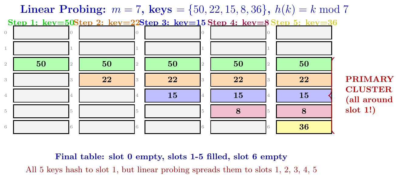
Primary clustering is the main problem with linear probing. When many keys hash to the same slot and create a cluster (a long continuous run of filled slots), future keys that hash anywhere in that cluster will have to probe past the entire cluster to find an empty slot. The cluster keeps growing, making future insertions and searches slower. This is a snowball effect: the larger the cluster, the more likely new keys land in it, making it even larger.
Quadratic Probing
In quadratic probing, instead of moving one step at a time, we move by quadratic distances. \[ h(k, i) = (h(k) + c_1 i + c_2 i^2) \bmod m, i = 0, 1, 2, \ldots \] A common simple form is $h(k, i) = (h(k) + i^2) \bmod m$.
So if $h(k) = 3$: try slot 3, then $3 + 1 = 4$, then $3 + 4 = 7$, then $3 + 9 = 12$, and so on (all modulo $m$).
This spreads out keys much better than linear probing, reducing primary clustering. But quadratic probing can still cause secondary clustering: two keys with the same initial hash always follow the same probe sequence.
Table size $m = 11$. $h(k) = k \bmod 11$. Insert keys $\{18, 26, 35, 9\}$.
$h(18) = 7 \to$ slot 7 empty. Insert at 7.
$h(26) = 4 \to$ slot 4 empty. Insert at 4.
$h(35) = 2 \to$ slot 2 empty. Insert at 2.
$h(9) = 9 \to$ slot 9 empty. Insert at 9.
Now insert 44: $h(44) = 0 \to$ slot 0 empty. Insert at 0.
Now insert 55: $h(55) = 0 \to$ slot 0 occupied! Try $i=1$: $(0 + 1) \bmod 11 = 1 \to$ empty. Insert at 1.
Now insert 66: $h(66) = 0 \to$ slot 0 occupied! Try $i=1$: slot 1 occupied. Try $i=2$: $(0+4)\bmod 11 = 4 \to$ occupied! Try $i=3$: $(0+9)\bmod 11 = 9 \to$ occupied! Try $i=4$: $(0+16)\bmod 11 = 5 \to$ empty. Insert at 5.
Secondary clustering occurs in quadratic probing. Two different keys that hash to the same initial slot $h(k)$ will follow the exact same probe sequence. So they always compete for the same set of slots. However, two keys with different initial hashes never follow the same sequence. This is less severe than primary clustering but still an issue.
Double Hashing
Double hashing uses a second hash function to determine the step size. \[ h(k, i) = (h_1(k) + i \cdot h_2(k)) \bmod m, i = 0, 1, 2, \ldots \] where $h_1$ and $h_2$ are two different hash functions. The step size $h_2(k)$ is different for different keys, so two keys that have the same $h_1(k)$ will likely have different $h_2(k)$ values, meaning they follow completely different probe sequences. This eliminates both primary and secondary clustering, and gives the best performance among open addressing methods.
Common choice: $h_1(k) = k \bmod m$ and $h_2(k) = 1 + (k \bmod (m-1))$. We ensure $h_2(k) \ne 0$ so we actually move forward.
Table size $m = 7$. $h_1(k) = k \bmod 7$, $h_2(k) = 1 + (k \bmod 6)$. Insert $\{18, 25, 35\}$.
Insert 18: $h_1(18) = 4 \to$ slot 4 empty. Insert at 4.
Insert 25: $h_1(25) = 4 \to$ slot 4 occupied! $h_2(25) = 1 + 25\bmod6 = 1+1 = 2$. Try $(4 + 1\times2)\bmod7 = 6 \to$ slot 6 empty. Insert at 6.
Insert 35: $h_1(35) = 0 \to$ slot 0 empty. Insert at 0.
Now insert 11: $h_1(11) = 4 \to$ occupied. $h_2(11) = 1+11\bmod6 = 1+5 = 6$. Try $(4+6)\bmod7 = 3 \to$ empty. Insert at 3. A different probe sequence from key 25 (even though both first went to slot 4).
class OpenAddressingHT:
    def __init__(self, m, method='linear'):
        self.m       = m
        self.table   = [None] * m
        self.deleted = [False] * m   # lazy deletion marker
        self.method  = method

    def h1(self, key):
        return key % self.m

    def h2(self, key):
        return 1 + (key % (self.m - 1))  # for double hashing

    def probe(self, key, i):
        if self.method == 'linear':
            return (self.h1(key) + i) % self.m
        elif self.method == 'quadratic':
            return (self.h1(key) + i*i) % self.m
        else:  # double hashing
            return (self.h1(key) + i * self.h2(key)) % self.m

    def insert(self, key):
        for i in range(self.m):
            slot = self.probe(key, i)
            if self.table[slot] is None or self.deleted[slot]:
                self.table[slot]   = key
                self.deleted[slot] = False
                return True
        print("Hash table is FULL")
        return False

    def search(self, key):
        for i in range(self.m):
            slot = self.probe(key, i)
            if self.table[slot] is None and not self.deleted[slot]:
                return False        # empty slot means key not present
            if self.table[slot] == key and not self.deleted[slot]:
                return True
        return False

    def delete(self, key):
        for i in range(self.m):
            slot = self.probe(key, i)
            if self.table[slot] is None and not self.deleted[slot]:
                return False
            if self.table[slot] == key and not self.deleted[slot]:
                self.deleted[slot] = True   # lazy deletion
                return True
        return False

    def display(self):
        for i, val in enumerate(self.table):
            status = "DEL" if self.deleted[i] else str(val)
            print(f"Slot {i}: {status}")


# --- Driver Code ---
print("=== Linear Probing ===")
ht = OpenAddressingHT(7, 'linear')
for key in [50, 22, 15, 8, 36]:
    ht.insert(key)
ht.display()

print("\n=== Double Hashing ===")
ht2 = OpenAddressingHT(7, 'double')
for key in [50, 22, 15, 8, 36]:
    ht2.insert(key)
ht2.display()
Performance Analysis
The performance of open addressing depends on the load factor $\alpha$. Under the assumption of uniform hashing, the expected number of probes for:
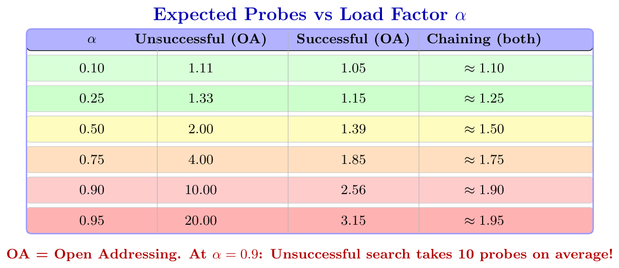
Unsuccessful Search (looking for a key that is NOT in the table): \[ \text{Expected probes} \le \frac{1}{1 - \alpha} \]
Successful Search (looking for a key that IS in the table): \[ \text{Expected probes} \le \frac{1}{\alpha} \ln \frac{1}{1-\alpha} \]
These formulas assume open addressing with uniform probing. For chaining, the analysis is different.
For chaining with load factor $\alpha = n/m$:
Unsuccessful Search: Expected number of elements examined = $\alpha$ (length of a randomly chosen chain), plus 1 for computing the hash. So total work is $\Theta(1 + \alpha)$.
Successful Search: Expected work is $\Theta(1 + \alpha)$.
Insert: $O(1)$ (insert at front of chain, plus computing hash).
Delete: $O(1 + \alpha)$ (find the element first, then delete).
When $\alpha = O(1)$ (load factor kept constant by resizing), all operations are $O(1)$.
Consider a hash table with $m = 10$ slots and $n = 7$ keys inserted. So $\alpha = 7/10 = 0.7$.
Open Addressing:
Expected probes for unsuccessful search $= \dfrac{1}{1-0.7} = \dfrac{1}{0.3} \approx 3.33$
Expected probes for successful search $\approx \dfrac{1}{0.7} \ln\dfrac{1}{0.3} \approx 1.43 \times 1.20 \approx 1.72$
Chaining:
Expected work $= \Theta(1 + 0.7) = \Theta(1.7)$, roughly 1.7 operations per search.
So at $\alpha = 0.7$, chaining is significantly more efficient than open addressing for unsuccessful search.
The load factor is the single most important tuning parameter of a hash table. Key observations:
For $\alpha \le 0.5$: open addressing is fast, with expected probes close to 2 or less.
For $\alpha > 0.7$: open addressing degrades significantly.
Chaining degrades gracefully because chains simply get longer, but the overhead is just the chain length.
Real-world hash tables are resized (rehashed) when $\alpha$ crosses a threshold, typically 0.7 for open addressing and around 1.0 for chaining.
Resizing means creating a new larger array and reinserting all keys. This costs $O(n)$ but happens infrequently, so amortized cost remains $O(1)$ per operation.
import math

def expected_probes_open_addressing(alpha):
    """Expected probes for open addressing (uniform hashing)"""
    if alpha >= 1:
        return float('inf')
    unsuccessful = 1 / (1 - alpha)
    successful   = (1 / alpha) * math.log(1 / (1 - alpha))
    return unsuccessful, successful


def expected_probes_chaining(alpha):
    """Expected probes for chaining"""
    unsuccessful = 1 + alpha
    successful   = 1 + alpha / 2
    return unsuccessful, successful


print(f"{'alpha':>6} | {'OA-Unsucc':>10} | {'OA-Succ':>9} | {'Chain-Unsucc':>12} | {'Chain-Succ':>10}")
print("-" * 65)
for alpha in [0.1, 0.25, 0.50, 0.75, 0.90, 0.95]:
    oa_u, oa_s   = expected_probes_open_addressing(alpha)
    ch_u, ch_s   = expected_probes_chaining(alpha)
    print(f"{alpha:>6.2f} | {oa_u:>10.2f} | {oa_s:>9.2f} | {ch_u:>12.2f} | {ch_s:>10.2f}")

# Output:
# alpha | OA-Unsucc |   OA-Succ | Chain-Unsucc | Chain-Succ
# ----------------------------------------------------------------
#  0.10 |      1.11 |      1.05 |         1.10 |       1.05
#  0.25 |      1.33 |      1.15 |         1.25 |       1.12
#  0.50 |      2.00 |      1.39 |         1.50 |       1.25
#  0.75 |      4.00 |      1.85 |         1.75 |       1.38
#  0.90 |     10.00 |      2.56 |         1.90 |       1.45
# 0.95 | 20.00 | 3.15 | 1.95 | 1.48Division method for hash function: simple, works well if $m$ is a prime not close to a power of 2.
Multiplication method: works well for any $m$, including powers of 2.
Chaining: easy to implement, handles $\alpha > 1$, graceful degradation, but uses extra memory for pointers.
Linear probing: best cache performance (sequential access), but primary clustering makes it slow at high $\alpha$.
Quadratic probing: reduces primary clustering, but secondary clustering remains, and not all slots guaranteed to be probed.
Double hashing: best performance among open addressing methods, avoids both types of clustering, but needs two hash functions.