Introduction to Machine Learning
What is Machine Learning
Machine Learning (ML) is the practice of building systems that improve their behaviour through experience (data). Instead of encoding exact rules for every case, ML systems detect patterns, form general rules from examples, and apply those rules to new situations. In simple terms: ML finds useful patterns in data and uses them to make predictions, decisions, or generate useful outputs.
Learning from examples: Provide examples that show input and desired output or let the system find structure in inputs alone.
Generalization: The ability to perform well on new, unseen examples that come from the same kind of data.
Feedback loop: The system improves when it receives signals telling it how well it did (explicit labels, rewards, or implicit signals like clicks).
Think of teaching a child to recognize apples. Rather than giving a strict rule ("red and round equals apple"), you show many examples (red apples, green apples, sliced apples). The child learns a flexible concept from examples and can correctly identify new apples despite differences in color, shape, or lighting.

Overview of Machine Learning Paradigm
ML development typically follows a repeatable loop:
Collect data relevant to the problem.
Preprocess and explore data to understand its structure.
Select or design an appropriate model architecture.
Train the model on the data (learn patterns).
Validate and evaluate on held-out examples.
Deploy and monitor in production and iterate with new data.

Iterating the loop allows improvement. Real-world ML rarely works on the first try — understanding data quirks, evaluating fairness, and updating models as environments change are essential steps in practical ML.
Types: supervised, unsupervised, and reinforcement learning
Supervised learning: Learn from examples where the desired outcome is given. Useful when labeled examples are available.
Unsupervised learning: Find structure in unlabeled data (grouping, representations).
Reinforcement learning: Learn to act through trial-and-error interactions with an environment using feedback in the form of rewards.
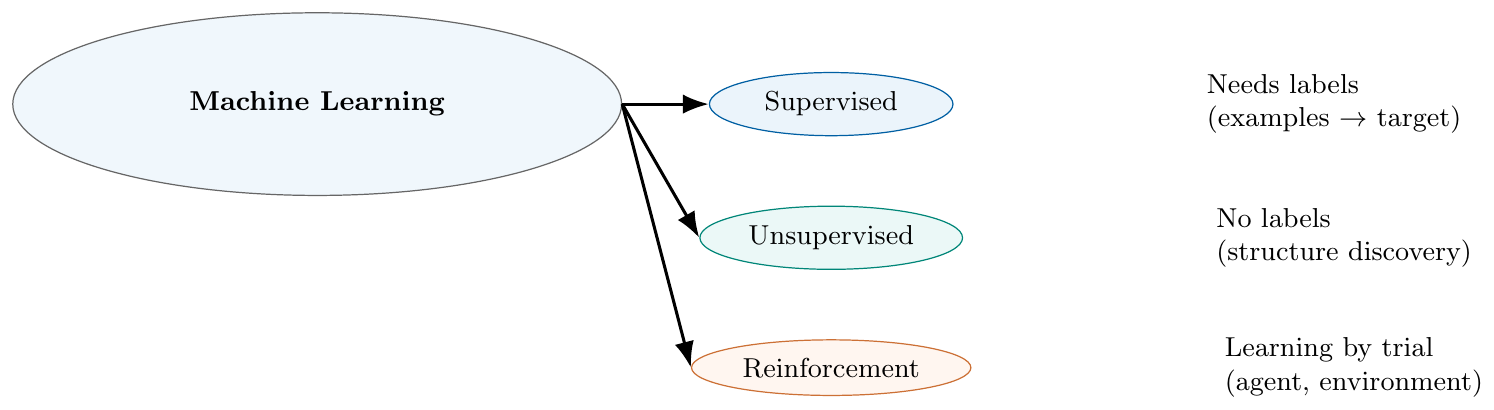
Supervised: Email labelled as "spam" or "not spam" → train a spam filter.
Unsupervised: Customer purchase histories → group (cluster) customers into segments for marketing.
Reinforcement: Robot learns to walk by trying actions and receiving rewards for forward progress and penalties for falling.
Data
Basic Types of Data
Tabular: Rows and columns (structured) — common in business data.
Text: Documents, chat logs, reviews — sequential and high-dimensional.
Images: Pixel grids with spatial structure.
Audio: Waveforms and spectrograms, temporal patterns.
Time-series: Measurements over time (stock prices, sensor readings).
Graphs: Entities connected by edges (social networks, molecules).
Different data types require different methods and preprocessing. For example, images benefit from convolutional approaches that exploit spatial locality; text needs tokenization and representations that handle order; graphs require methods that use connectivity structure.
Exploring Structure of Data
Before building models you must understand:
What features exist and their distributions.
Which features are noisy, missing, or correlated.
Whether labels (if any) are balanced or skewed.
Which exploratory visualizations reveal structure (histograms, scatter plots, example images).

Data Quality
Completeness: Are important values missing?
Consistency: Do records contradict each other?
Accuracy: Do values reflect reality or measurement error?
Timeliness: Are data current and relevant?
Representativeness: Does the data capture the population you care about?
Inspect missing values and patterns of missingness.
Check for duplicated records.
Validate ranges (dates, values) and enforce constraints.
Sample labels for human verification if labels are noisy.
Consider whether historical data reflects the present.
Data Pre-Processing
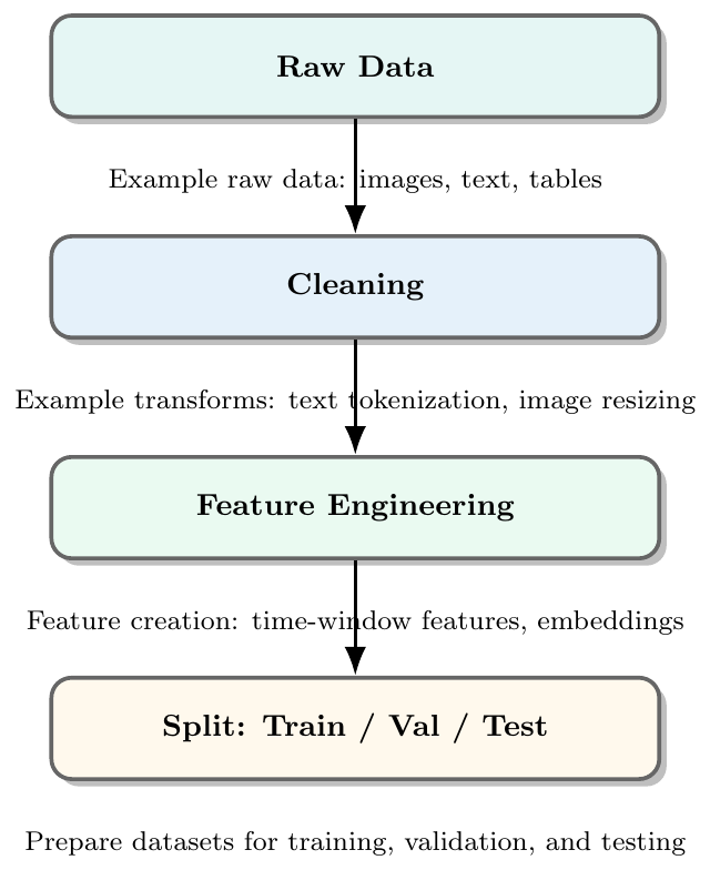
Before training, data is commonly cleaned and transformed:
Cleaning: remove or fix corrupted records, handle missing values.
Normalization / scaling: make ranges consistent where needed.
Encoding: transform categorical variables into numerical representations.
Feature creation: derive higher-level features from raw inputs.
Splitting: keep holdout data for fair evaluation (validation / test).
Parametric and Non-Parametric Functions
Parametric Functions
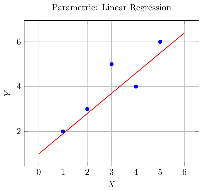
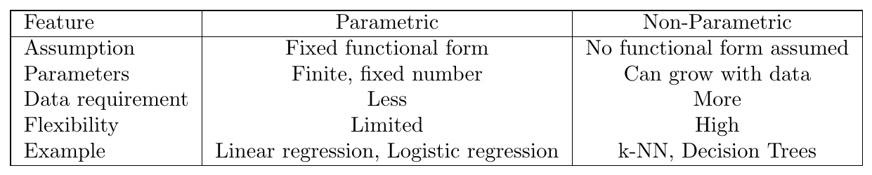
Parametric models assume a specific functional form for the relationship between input features $X$ and output $Y$, characterized by a finite set of parameters $\theta$.
\[ Y = f(X; \theta) \]
Key Points:
Requires assumption about the underlying distribution or functional form (e.g., linear, polynomial).
Number of parameters is fixed and does not depend on the number of training samples.
Learning reduces to estimating the parameters $\theta$ from data.
Examples: Linear regression, Logistic regression, Polynomial regression.
Simple linear regression:
\[ Y = \beta_0 + \beta_1 X + \epsilon \]
Here, the model is linear, and we estimate only $\beta_0$ (intercept) and $\beta_1$ (slope). Predictions for new $X$ values are made using these parameters.
Logistic regression:
\[ P(Y=1 \mid X) = \frac{1}{1 + e^{-(\beta_0 + \beta_1 X)}} \]
The model is parametric, with parameters $\beta_0$ and $\beta_1$ controlling the sigmoid function shape.
Non-Parametric Functions
Non-parametric models do not assume a fixed functional form. Instead, they learn the function directly from data.
Key Points:
Model complexity can grow with the dataset.
Often requires more data to avoid overfitting.
Can capture complex, nonlinear relationships.
Examples: k-Nearest Neighbors (k-NN), Decision Trees, Kernel Density Estimation.
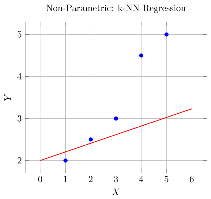
k-NN regression predicts the value at $X=x$ as the average of $Y$ values of the $k$ nearest neighbors:
\[ \hat{Y}(x) = \frac{1}{k} \sum_{i \in \mathcal{N}_k(x)} Y_i \]
No explicit parameters are estimated; predictions depend entirely on the data points.
Decision trees split the feature space into regions. For features $X_1$ and $X_2$:
\[ Y = \begin{cases} 5 & \text{if } X_1 < 3 \text{ and } X_2 > 2 \\ 7 & \text{if } X_1 \ge 3 \\ \end{cases} \]
The function form emerges from the splits, not predefined parameters.
Comparison: Parametric vs Non-Parametric
Issues in ML
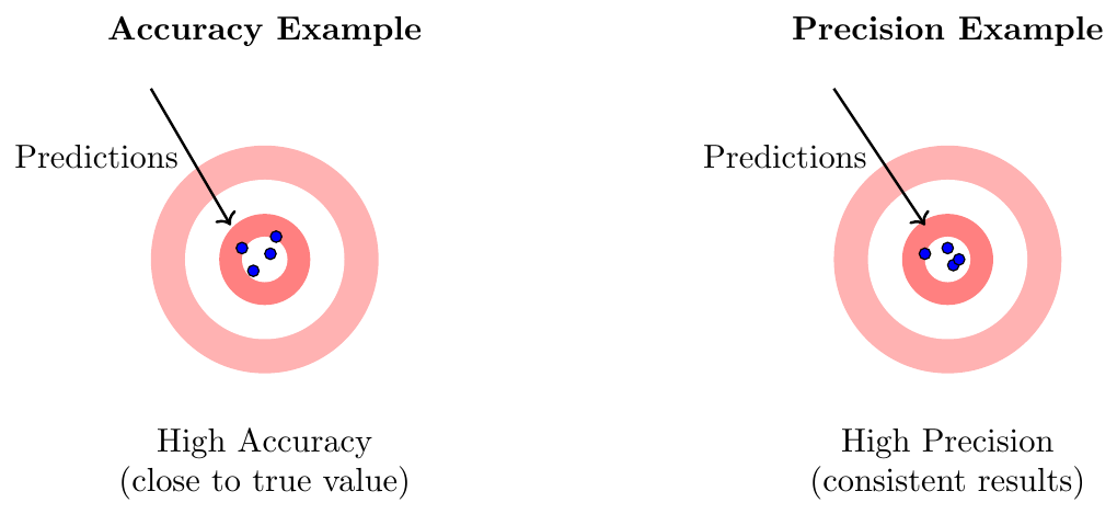
Accuracy and Precision
Accuracy: Is the model giving the correct results overall (close to true value)?
Precision: MIs the model consistent in giving the same correct result each time (consistent results)?
Issues
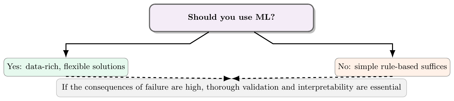
ML is powerful, but it is not always the best tool. Avoid ML when:
The task can be solved reliably with deterministic rules or simple logic.
You lack sufficient, representative data covering real-world variability.
You need fully explainable, provably-correct behaviour for safety-critical tasks (unless the ML system has been heavily validated).
Data privacy, legal, or ethical constraints prevent the collection or usage of the required data.
Bias in data: Historical biases in training data lead to biased outputs.
Concept drift: Data distributions change over time; models must be updated.
Overfitting: Model learns noise or dataset quirks that don't generalize.
Underfitting: Model is too simple to capture important structure.
Interpretability: Some models (deep nets) are harder to explain.
Definition: Data bias occurs when the training data does not fairly represent the real-world population. This leads the model to make systematically unfair or inaccurate predictions.
Example: A hiring model is trained mostly on male applicants. When used for new applicants, it prefers male candidates even with identical qualifications.
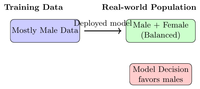
Consequence: The model generalizes poorly across groups, causing unfair treatment or legal risks.
Definition: Concept drift occurs when the relationship between input features and output labels changes over time.
Example: A credit card fraud detection system trained in 2018 fails in 2025 because fraud patterns evolve.
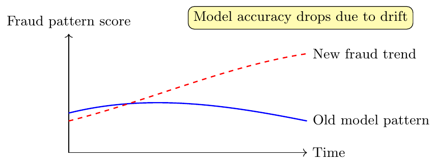
Consequence: Models degrade unless retrained periodically with new data.
Definition: Overfitting happens when the model learns both the true pattern and the noise of the training set, performing poorly on unseen data.
Example: A decision tree memorizes every training example, achieving 100% accuracy on training but 60% on test data.
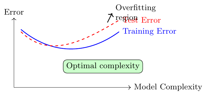
Consequence: Model appears perfect during training but fails in real applications.
Definition: Underfitting occurs when a model is too simple to capture the true underlying pattern in data.
Example: Using a straight line to model a quadratic relationship \( y = x^2 \).
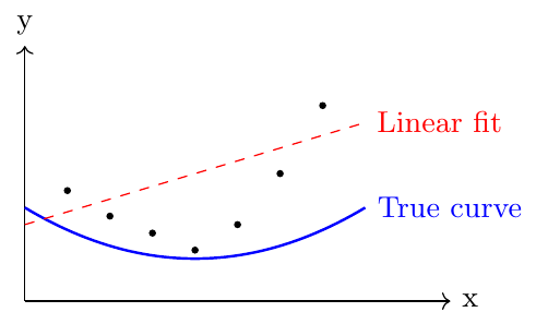
Consequence: Both training and test accuracy remain poor due to model simplicity.
Definition: Interpretability means understanding why a model makes certain predictions. Complex models like deep neural networks are powerful but often opaque.
Example: A CNN classifies an image as “dog”, but we don’t know which pixels or regions influenced the decision.

Consequence: Lack of interpretability makes debugging, fairness evaluation, and trust difficult.
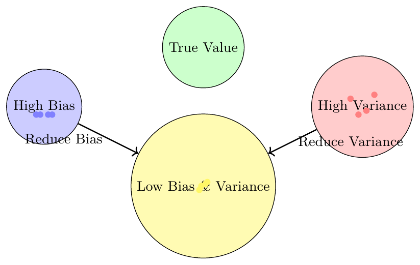
Bias and Variance
In any predictive task, the model's error can be understood as a combination of three components:
Bias: The systematic error introduced by approximating a complex problem with a simplified model. High bias implies the model consistently misses the target in a certain direction.
Variance: The error due to sensitivity to small changes in the training data. High variance implies the model's predictions fluctuate a lot when data changes.
Irreducible noise: Random variability in the system or inherent unpredictability.
The total expected error at a point $x$ can be decomposed as:
\[ \mathbb{E}[(\hat{f}(x) - f(x))^2] = \underbrace{(\text{Bias}[\hat{f}(x)])^2}_{\text{Squared Bias}} + \underbrace{\text{Var}[\hat{f}(x)]}_{\text{Variance}} + \underbrace{\sigma^2}_{\text{Irreducible Noise}} \]
Suppose we try to predict a quantity $y$ multiple times using a model and obtain these predictions:
\[ \hat{y}_1 = 5.2, \quad \hat{y}_2 = 4.9, \quad \hat{y}_3 = 5.1 \]
The true value is $y = 5$.
Bias: Average difference between predictions and true value: \[ \text{Bias} = \bar{\hat{y}} - y = \frac{5.2 + 4.9 + 5.1}{3} - 5 = 5.067 - 5 = 0.067 \]
Variance: Spread of predictions around their mean: \[ \text{Variance} = \frac{(5.2-5.067)^2 + (4.9-5.067)^2 + (5.1-5.067)^2}{3} \approx 0.0089 \]
Total Error: Bias$^2$ + Variance: \[ \text{Error} \approx 0.067^2 + 0.0089 \approx 0.0133 \]
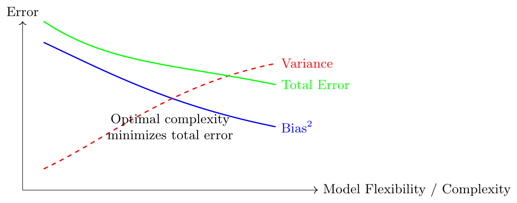
A simple constant model predicting the average: High bias, low variance.
A model that outputs random predictions: Low bias on average, high variance.
Averaging several independent models: Reduces variance without increasing bias.
Overly simplistic formula for forecasting: High bias, may underfit data.
Highly sensitive formula reacting to every minor fluctuation: Low bias, high variance.
Evaluation Metrics for Classification
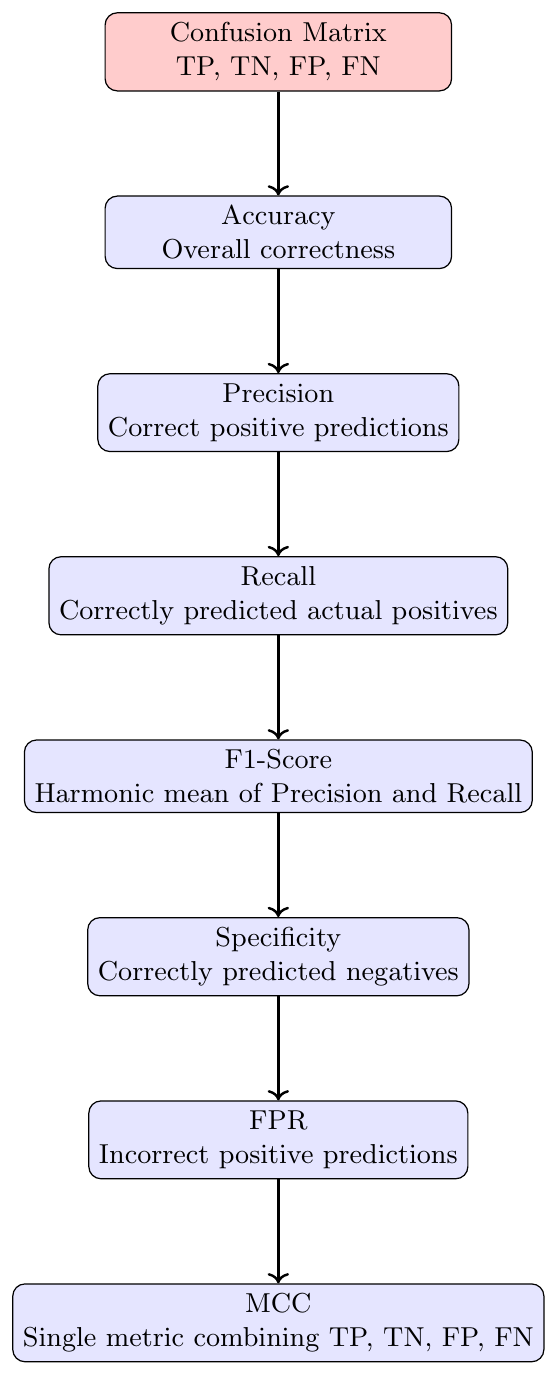
Classification metrics evaluate the performance of supervised learning models by measuring how well predicted labels match actual labels.
They are derived from the confusion matrix, which summarizes predictions:
True Positive (TP): Correctly predicted positive class.
False Positive (FP): Incorrectly predicted positive class.
True Negative (TN): Correctly predicted negative class.
False Negative (FN): Incorrectly predicted negative class.

This matrix forms the basis for computing all classification metrics.
Accuracy measures the overall correctness of the model:
\[ \text{Accuracy} = \frac{TP + TN}{TP + TN + FP + FN} \]
Example: TP=40, TN=50, FP=5, FN=5
\[ \text{Accuracy} = \frac{40+50}{40+50+5+5} = 0.9 = 90\% \]
Precision measures how many predicted positives are actually positive:
\[ \text{Precision} = \frac{TP}{TP + FP} \]
Example: TP=40, FP=5
\[ \text{Precision} = \frac{40}{40+5} \approx 0.8889 = 88.89\% \]
High precision indicates few false positives.
Recall measures how many actual positives were correctly predicted:
\[ \text{Recall} = \frac{TP}{TP + FN} \]
Example: TP=40, FN=5
\[ \text{Recall} = \frac{40}{40+5} \approx 0.8889 = 88.89\% \]
High recall indicates few false negatives.
F1-Score is the harmonic mean of Precision and Recall:
\[ \text{F1} = 2 \cdot \frac{\text{Precision} \cdot \text{Recall}}{\text{Precision} + \text{Recall}} \]
Example: Precision=0.8889, Recall=0.8889
\[ \text{F1} = 2 \cdot \frac{0.8889 \cdot 0.8889}{0.8889+0.8889} = 0.8889 = 88.89\% \] It balances Precision and Recall.
Specificity measures how many actual negatives were correctly predicted:
\[ \text{Specificity} = \frac{TN}{TN + FP} \]
Example: TN=50, FP=5
\[ \text{Specificity} = \frac{50}{50+5} \approx 0.909 = 90.9\% \]
FPR measures incorrect positive predictions:
\[ \text{FPR} = \frac{FP}{FP + TN} = 1 - \text{Specificity} \]
Example: FP=5, TN=50
\[ \text{FPR} = \frac{5}{50+5} \approx 0.0909 = 9.09\% \]
MCC combines TP, TN, FP, FN into a single metric:
\[ \text{MCC} = \frac{TP \cdot TN - FP \cdot FN}{\sqrt{(TP+FP)(TP+FN)(TN+FP)(TN+FN)}} \]
Example: TP=40, TN=50, FP=5, FN=5
\[ \text{MCC} = \frac{40\cdot50 - 5\cdot5}{\sqrt{(40+5)(40+5)(50+5)(50+5)}} \approx 0.889 \]
MCC ranges from -1 (worst) to 1 (perfect prediction).
Suppose we have a dataset of 20 patients where a model predicts whether each patient has a disease (Positive) or not (Negative).
The predictions vs actual outcomes are summarized as:

From this confusion matrix:
True Positives (TP) = 6
False Negatives (FN) = 2
False Positives (FP) = 3
True Negatives (TN) = 9
Now we calculate the common metrics:
\[ \text{Accuracy} = \frac{TP+TN}{TP+TN+FP+FN} = \frac{6+9}{6+9+3+2} = \frac{15}{20} = 0.75 = 75\% \]
\[ \text{Precision} = \frac{TP}{TP+FP} = \frac{6}{6+3} = \frac{6}{9} \approx 0.667 = 66.7\% \]
\[ \text{Recall (Sensitivity)} = \frac{TP}{TP+FN} = \frac{6}{6+2} = \frac{6}{8} = 0.75 = 75\% \]
\[ \text{F1-Score} = 2 \cdot \frac{\text{Precision} \cdot \text{Recall}}{\text{Precision} + \text{Recall}} = 2 \cdot \frac{0.667 \cdot 0.75}{0.667+0.75} \approx 0.706 = 70.6\% \]
\[ \text{Specificity} = \frac{TN}{TN+FP} = \frac{9}{9+3} = \frac{9}{12} = 0.75 = 75\% \]
\[ \text{False Positive Rate (FPR)} = \frac{FP}{FP+TN} = \frac{3}{3+9} = \frac{3}{12} = 0.25 = 25\% \]
A multi-class classifier (4 classes) is evaluated on 400 samples. The confusion matrix is partially given:
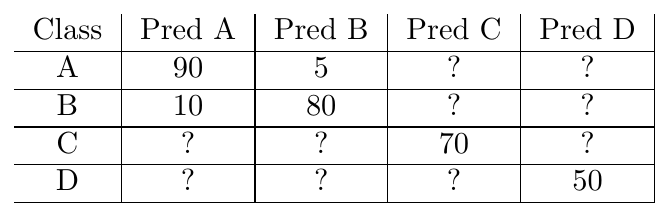
Fill missing entries assuming total samples per class: A=100, B=100, C=100, D=100. Compute per-class Precision, Recall, and macro-F1.
Solution:
We are given each row's total = 100. We'll fill missing entries by distributing each row's remaining misclassifications across the unknown predicted columns. (Any reasonable integer allocation that makes each row sum to 100 is acceptable — here we use a simple balanced distribution; explainable choices are fine in exam settings.)
Fill rows (one possible integer allocation):
Row A: known 90 (Pred A) + 5 (Pred B) = 95, remainder 5 → distribute as Pred C = 3, Pred D = 2.
Row B: known 10 (Pred A) + 80 (Pred B) = 90, remainder 10 → Pred C = 5, Pred D = 5.
Row C: known 70 (Pred C), remainder 30 → distribute Pred A = 10, Pred B = 10, Pred D = 10.
Row D: known 50 (Pred D), remainder 50 → distribute Pred A = 17, Pred B = 17, Pred C = 16 (sums to 50).
So the completed confusion matrix (Actual rows, Predicted columns):
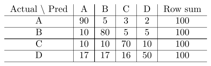
Column sums (predicted counts): \[ \text{Pred A} = 90+10+10+17 = 127 \] \[ \text{Pred B} = 5+80+10+17 = 112 \] \[ \text{Pred C} = 3+5+70+16 = 94 \] \[ \text{Pred D} = 2+5+10+50 = 67 \]
Now compute per-class metrics (for class \(\text{X}\): TP = diagonal entry, Precision = TP / (predicted X column sum), Recall = TP / 100 (actual class size)).
Class A: \[ \text{TP}_A = 90,\quad \text{Precision}_A = \frac{90}{127}\approx 0.7087 \; (70.87\%),\quad \text{Recall}_A = \frac{90}{100}=0.9\; (90\%). \] F1\(_A\) \(= 2\cdot \frac{0.7087\cdot 0.9}{0.7087+0.9}\approx 0.7930\) (79.30%).
Class B: \[ \text{TP}_B = 80,\quad \text{Precision}_B = \frac{80}{112}\approx 0.7143\; (71.43\%),\quad \text{Recall}_B = \frac{80}{100}=0.8\; (80\%). \] F1\(_B\) \(\approx 0.7547\) (75.47%).
Class C: \[ \text{TP}_C = 70,\quad \text{Precision}_C = \frac{70}{94}\approx 0.7447\; (74.47\%),\quad \text{Recall}_C = \frac{70}{100}=0.7\; (70\%). \] F1\(_C\) \(\approx 0.7216\) (72.16%).
Class D: \[ \text{TP}_D = 50,\quad \text{Precision}_D = \frac{50}{67}\approx 0.7463\; (74.63\%),\quad \text{Recall}_D = \frac{50}{100}=0.5\; (50\%). \] F1\(_D\) \(\approx 0.5988\) (59.88%).
Macro-F1: average of per-class F1s: \[ \text{Macro-F1} = \frac{0.7930 + 0.7547 + 0.7216 + 0.5988}{4} \approx 0.7170 \; (71.70\%). \]
Interpretation: - Recalls show class A is recognized very well (90%), class D lags (50%). - Precision values are roughly similar (71–75%), but class D’s low recall penalizes its F1. - If you need to prioritize a particular class (say D), adjust model or collect more data for that class.
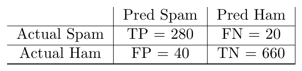
A machine learning model classifies emails as spam or ham. Out of 1000 emails: 300 spam, 700 ham. The model predicts 280 spam correctly, 40 ham as spam, 20 spam as ham, and remaining correctly as ham. Compute Accuracy, Precision, Recall, F1, Specificity, and MCC.
Solution:
First derive confusion-matrix entries:
Actual positive (spam) = 300. Model predicts 280 correctly \(\Rightarrow\) TP = 280.
Among spam, 20 predicted ham \(\Rightarrow\) FN = 20.
Model mislabels 40 ham as spam \(\Rightarrow\) FP = 40.
Remaining ham correctly predicted: TN = total ham - FP = 700 - 40 = 660.
Confusion matrix:
Now compute metrics:
\[ \text{Accuracy} = \frac{TP + TN}{\text{Total}} = \frac{280 + 660}{1000} = \frac{940}{1000} = 0.94 = 94\%. \]
\[ \text{Precision} = \frac{TP}{TP + FP} = \frac{280}{280 + 40} = \frac{280}{320} = 0.875 = 87.5\%. \]
\[ \text{Recall} = \frac{TP}{TP + FN} = \frac{280}{280 + 20} = \frac{280}{300} \approx 0.9333 = 93.33\%. \]
\[ \text{F1} = 2\cdot\frac{\text{Precision}\cdot\text{Recall}}{\text{Precision}+\text{Recall}} = 2\cdot\frac{0.875\cdot 0.9333}{0.875 + 0.9333} \approx 0.9032 = 90.32\%. \]
\[ \text{Specificity} = \frac{TN}{TN + FP} = \frac{660}{660 + 40} = \frac{660}{700} \approx 0.9429 = 94.29\%. \]
\[ \text{MCC} = \frac{TP\cdot TN - FP\cdot FN}{\sqrt{(TP+FP)(TP+FN)(TN+FP)(TN+FN)}} = \frac{280\cdot660 - 40\cdot20}{\sqrt{(320)(300)(700)(680)}} \approx 0.8608. \]
Interpretation: High accuracy and recall show the model catches most spam; precision < recall means of all predicted spam, some fraction are false alarms. MCC \(\approx 0.86\) indicates strong overall classification quality accounting for all four cells.
A rare event detection model evaluates 50{,}000 events. Only 100 are positive. The model flags 120 events as positive, including 90 true positives. Compute FPR, Precision, Recall, and discuss the effect of class imbalance.
Solution:
From problem statement: \[ \text{Total positives} = 100,\quad TP = 90,\quad \text{model flagged positives} = 120 \Rightarrow FP = 120 - 90 = 30. \] \[ \text{Total negatives} = 50{,}000 - 100 = 49{,}900,\quad TN = 49{,}900 - FP = 49{,}900 - 30 = 49{,}870. \]
Compute metrics:
\[ \text{Precision} = \frac{TP}{TP+FP} = \frac{90}{90+30} = \frac{90}{120} = 0.75 = 75\%. \]
\[ \text{Recall} = \frac{TP}{TP+FN} = \frac{90}{100} = 0.9 = 90\%. \]
\[ \text{False Positive Rate (FPR)} = \frac{FP}{FP+TN} = \frac{30}{30 + 49{,}870} = \frac{30}{49{,}900} \approx 0.0006012 \approx 0.06012\%. \]
Discussion (class imbalance):
The recall (90%) and precision (75%) are fairly good. However, even a tiny FPR (0.06%) can produce many false positives when the dataset is huge. Here FP=30 is small in absolute terms — but if the negative population were even larger or the FPR slightly higher, false positives would grow quickly.
In rare-event detection, Precision and FPR are critical: a low FPR is necessary to avoid an overwhelming number of false alarms. Also consider metrics like Precision-Recall curve or use specialized loss/thresholding to control FP.
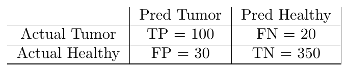
A medical imaging system detects tumors in CT scans. Out of 500 scans, 120 contain tumors. The system correctly identifies 100 tumors and misclassifies 30 healthy scans. Compute Accuracy, Precision, Recall, F1, and suggest which metric should guide deployment.
Solution:
Given: \[ \text{Total scans} = 500,\quad \text{Positives (tumor)} = 120,\quad TP = 100,\quad FP = 30. \] Compute remaining cells: \[ FN = 120 - 100 = 20, \] \[ \text{Negatives} = 500 - 120 = 380,\quad TN = 380 - FP = 380 - 30 = 350. \]
Confusion matrix:
Metrics:
\[ \text{Accuracy} = \frac{TP + TN}{500} = \frac{100 + 350}{500} = \frac{450}{500} = 0.9 = 90\%. \]
\[ \text{Precision} = \frac{100}{100 + 30} = \frac{100}{130} \approx 0.7692 = 76.92\%. \]
\[ \text{Recall (Sensitivity)} = \frac{100}{100 + 20} = \frac{100}{120} \approx 0.8333 = 83.33\%. \]
\[ \text{F1} = 2\cdot \frac{0.7692 \cdot 0.8333}{0.7692 + 0.8333} \approx 0.8000 = 80.00\%. \]
Which metric should guide deployment?
In medical detection tasks, missing a true positive (i.e., a tumor) can have severe consequences. Thus Recall (sensitivity) is often the top priority — we want to minimize FN. An acceptable approach is to maximize recall while keeping precision at an operationally acceptable level (to avoid overwhelming radiologists with false positives).
However, extremely low precision (many false positives) will create excessive follow-ups and costs; so balance is needed — use recall as priority with constraints on acceptable precision. Use ROC / Precision-Recall curves for threshold selection, and engage clinical stakeholders to set acceptable trade-offs.
A social media model detects offensive posts. Out of 10{,}000 posts, 200 are offensive. The model flags 180 correctly, but 400 normal posts as offensive. Compute confusion matrix, Precision, Recall, F1-score, and MCC.
Solution:
Given: \[ \text{Total} = 10{,}000,\quad \text{Positives (offensive)} = 200,\quad TP = 180,\quad FP = 400. \] Then: \[ FN = 200 - 180 = 20. \] Negatives: \[ \text{Negatives} = 10{,}000 - 200 = 9{,}800,\quad TN = 9{,}800 - 400 = 9{,}400. \]
Confusion matrix:

Compute metrics:
\[ \text{Precision} = \frac{TP}{TP+FP} = \frac{180}{180 + 400} = \frac{180}{580} \approx 0.3103 = 31.03\%. \]
\[ \text{Recall} = \frac{TP}{TP+FN} = \frac{180}{180 + 20} = \frac{180}{200} = 0.9 = 90\%. \]
\[ \text{F1} = 2\cdot\frac{0.3103 \cdot 0.9}{0.3103 + 0.9} \approx 0.4615 = 46.15\%. \]
\[ \text{MCC} = \frac{TP\cdot TN - FP\cdot FN}{\sqrt{(TP+FP)(TP+FN)(TN+FP)(TN+FN)}} = \frac{180\cdot9400 - 400\cdot20}{\sqrt{(580)(200)(9800)(9200)}} \approx 0.5146. \]
Interpretation:
High recall (90%) — the model catches most offensive posts.
Low precision (31%) — many false positives, so moderation teams will see many normal posts flagged.
F1 around 46% shows overall balance is poor due to low precision. MCC \(\approx 0.51\) indicates moderate classification performance accounting for imbalance.
For production, consider raising threshold, filtering, or a human-in-loop to reduce false positives; also consider cost of false positives vs false negatives for policy decisions.
Applications
Machine Learning powers many modern services and systems: search, recommendations, voice assistants, medical imaging, fraud detection, personalized education, robotics, weather forecasting, and many more. The value comes from converting raw or structured data into predictions, insights, or actions that support human decisions or automate tasks.
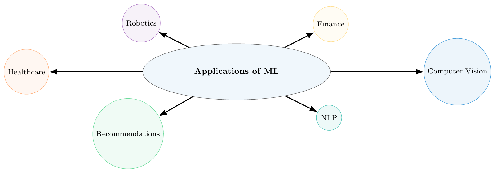
Computer Vision: Detect objects in images to help autonomous vehicles or medical image analysis to highlight abnormal tissue.
NLP: Translate languages, summarize documents, or extract information from text.
Recommendations: Suggest relevant products, songs, or videos by learning user preferences.
Healthcare: Predict patient risk and assist diagnostics (requires domain validation).
Finance: Detect fraudulent transactions or forecast market signals (with caution).