Regression & Classification Models
Decision Trees
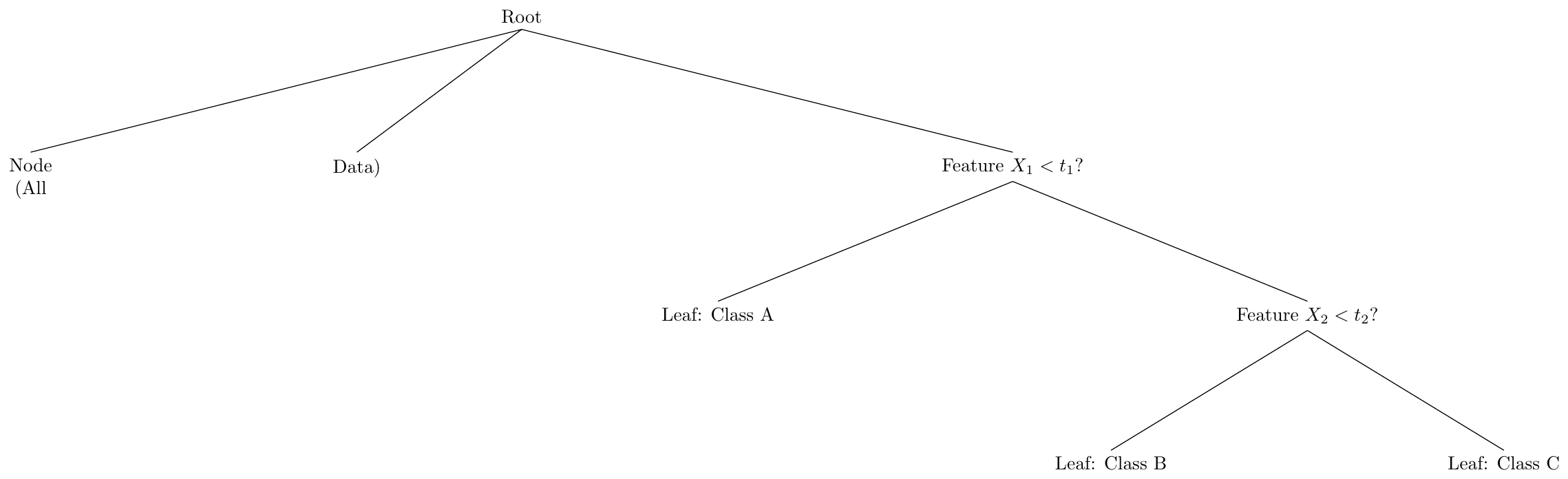
Decision Trees are non-parametric supervised learning models used for both classification and regression tasks. They work by recursively splitting the data space into homogeneous subsets based on feature values, forming a tree-like structure.
A Decision Tree consists of:
Root Node: Represents the entire dataset.
Internal Nodes: Represent decisions based on feature tests.
Leaf Nodes: Represent class labels (in classification) or continuous values (in regression).
Entropy, Gini Index, and Information Gain
Decision Trees divide data into smaller, purer subsets. To decide the best attribute for splitting, the tree evaluates impurity measures such as Shannon Entropy (ID3, C4.5) and Gini Index (CART). The attribute giving the maximum reduction in impurity is chosen.
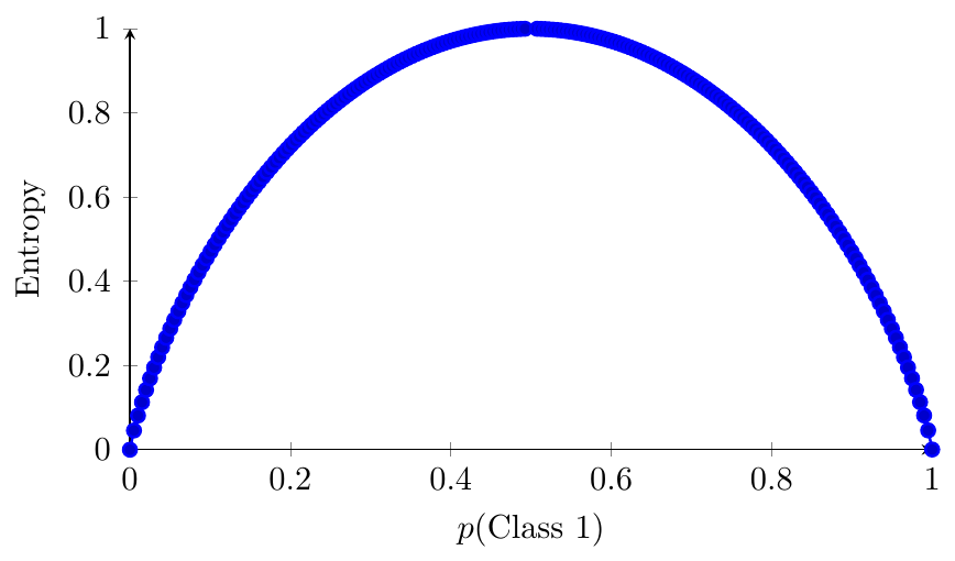
Entropy (from information theory) quantifies the uncertainty or disorder in a dataset.
\[ H(S) = - \sum_{i=1}^{k} p_i \log_2 p_i \]
where
$k$ = number of classes
$p_i$ = proportion of samples belonging to class $i$
Interpretation:
$H(S)=0$ when the dataset is pure (all samples belong to one class).
Entropy is maximum when classes are equally likely.
A dataset has 8 samples: 5 belong to Class A and 3 belong to Class B.
\[ H(S) = -\left( \frac{5}{8}\log_2\frac{5}{8} + \frac{3}{8}\log_2\frac{3}{8} \right) \]
\[ H(S) = -(0.625 \log_2 0.625 + 0.375 \log_2 0.375) = 0.954 \]
This indicates moderate impurity.
Gini Index (used in CART) measures the probability of a random sample being incorrectly classified.
\[ Gini(S) = 1 - \sum_{i=1}^{k} p_i^2 \]
Interpretation:
$Gini = 0$ means pure node.
Lower Gini indicates a better split.
Using the same dataset: 5 in Class A, 3 in Class B,
\[ Gini(S) = 1 - \left( \left(\frac{5}{8}\right)^2 + \left(\frac{3}{8}\right)^2 \right) \]
\[ Gini = 1 - (0.3906 + 0.1406) = 0.4688 \]
The node has moderate impurity.
Entropy uses logarithmic measure, Gini uses squared probabilities.
Both rank splits similarly in most cases.
Gini is computationally simpler (preferred in CART).
Information Gain quantifies the reduction in impurity after splitting on a feature.
\[ IG(S, A) = Impurity(S) - \sum_{v \in Values(A)} \frac{|S_v|}{|S|} \; Impurity(S_v) \]
Notes:
For ID3/C4.5: use Entropy in the formula.
For CART: use Gini Index.
A dataset has 10 samples: 6 in Class 1, 4 in Class 2.
\[ H(S) = - \left( \frac{6}{10}\log_2\frac{6}{10} + \frac{4}{10}\log_2\frac{4}{10} \right) = 0.971 \]
A feature splits the dataset into two subsets:
\[ S_1: 4 \text{ samples}, \quad H_1 = 0.5 \] \[ S_2: 6 \text{ samples}, \quad H_2 = 0.811 \]
Weighted entropy:
\[ H_{\text{split}} = \frac{4}{10}\times 0.5 + \frac{6}{10}\times 0.811 = 0.847 \]
Information Gain:
\[ IG = 0.971 - 0.847 = 0.124 \]
Thus, this feature gives an improvement of 0.124 in purity.
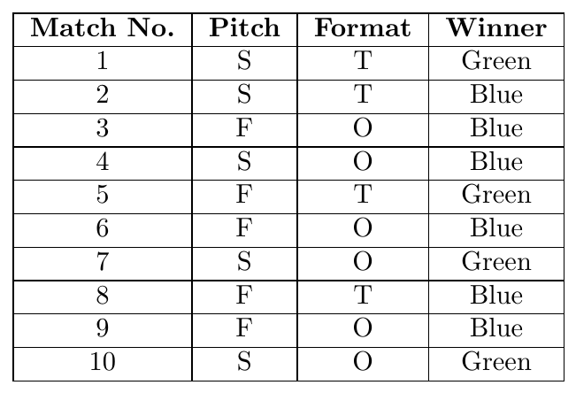
Table C: Details of cricket games between Green and Blue
Details of ten international cricket games between two teams “Green” and “Blue” are given in Table C. The attribute Pitch can take one of two values: spin-friendly (S) or pace-friendly (F). The attribute Format can take values: one-day (O) or test (T). The target variable is the Winner.
Compute the Information Gain $\text{IG(C, Pitch)}$ with respect to the Target.
Give the answer rounded to two decimal places.
Total matches = 10
Green wins = 4 Blue wins = 6
\[ H(\text{Winner}) = -\frac{4}{10}\log_2\left(\frac{4}{10}\right) -\frac{6}{10}\log_2\left(\frac{6}{10}\right) \]
\[ H(\text{Winner}) = -0.4\log_2(0.4) - 0.6\log_2(0.6) = 0.97095 \text{ bits} \]
Step 2: Entropy for each value of Pitch
Pitch = S (Spin-friendly)
Matches: 1,2,4,7,10 Green = 3, Blue = 2
\[ H(\text{Winner}|\text{Pitch}=S) = -\frac{3}{5}\log_2\left(\frac{3}{5}\right) -\frac{2}{5}\log_2\left(\frac{2}{5}\right) \]
\[ = -0.6\log_2(0.6) - 0.4\log_2(0.4) = 0.97095 \]
Pitch = F (Pace-friendly)
Matches: 3,5,6,8,9 Green = 1, Blue = 4
\[ H(\text{Winner}|\text{Pitch}=F) = -\frac{1}{5}\log_2\left(\frac{1}{5}\right) -\frac{4}{5}\log_2\left(\frac{4}{5}\right) \]
\[ = -0.2\log_2(0.2) - 0.8\log_2(0.8) = 0.72193 \]
Step 3: Conditional Entropy
\[ H(\text{Winner}|\text{Pitch}) = \frac{5}{10}(0.97095) + \frac{5}{10}(0.72193) \]
\[ = 0.84644 \]
Step 4: Information Gain
\[ \mathrm{IG}(C,\text{Pitch}) = H(\text{Winner}) - H(\text{Winner}|\text{Pitch}) \]
\[ = 0.97095 - 0.84644 = 0.12451 \]
\[ \boxed{\mathrm{IG}(C,\text{Pitch}) \approx 0.12} \]
Tree Construction and Stopping Criteria
Start with all training samples at the root.
Compute impurity (Entropy or Gini).
For each feature, calculate Information Gain.
Split on the feature with the highest IG.
Repeat recursively until:
Node is pure (all samples same class), or
Maximum depth reached, or
Minimum number of samples per node is met.
Consider features: \[ \text{Outlook: Sunny, Overcast, Rain}, \quad \text{Target: Play Tennis?} \] Compute $IG$ for each feature; the one with the highest gain (say, Outlook) becomes the root node. Repeat for child nodes recursively.
—
Tree Pruning and Overfitting
A large tree can overfit—capturing noise instead of true structure.
Pre-pruning: Stop growing tree early (limit depth, min samples).
Post-pruning: Grow full tree, then remove branches that do not improve validation accuracy.
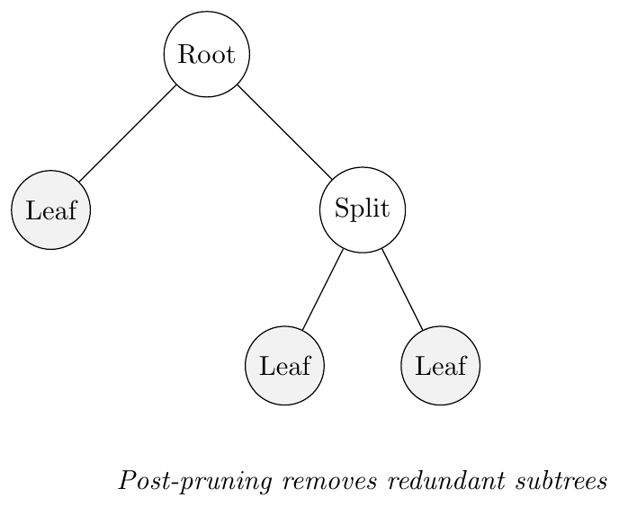
Reasoning: Pruning improves generalization by reducing variance. The goal is to find the simplest model that performs well on unseen data.
—
Bias–Variance Characteristics
Small trees: High bias, low variance (underfitting).
Large trees: Low bias, high variance (overfitting).
Ensemble methods (Random Forests): Reduce variance while maintaining low bias.
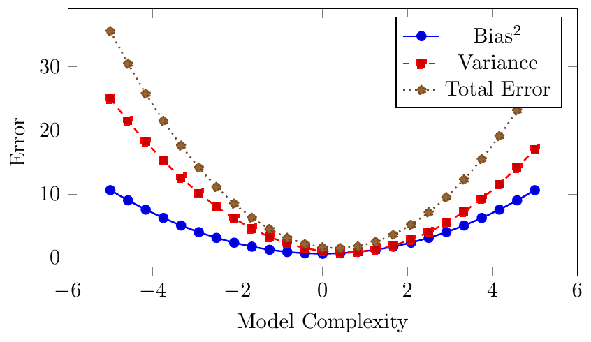
Insight: Decision Trees are powerful but unstable learners. Small changes in training data can drastically change splits. Ensembles like Random Forests or Gradient Boosted Trees help stabilize performance.
If a Decision Tree trained on a dataset of 100 samples achieves 100% accuracy on training but only 60% on test data, it exhibits:
Low bias (fits training perfectly)
High variance (poor generalization)
Using pruning or Random Forest can reduce variance.

}
Comparison of ID3, C4.5, and CART Algorithms
Support Vector Machine (SVM)
Introduction
Support Vector Machine (SVM) is a supervised learning algorithm grounded in statistical learning theory and Vapnik–Chervonenkis (VC) theory, primarily used for classification and regression tasks. In its most fundamental form, SVM is designed to construct an optimal decision boundary that best separates data points belonging to different classes.
SVM emphasizes the concept of margin maximization, wherein the separation boundary is chosen not merely to classify correctly, but to be as far as possible from the nearest training points of both classes, thereby enhancing generalization performance.
Throughout this section, we restrict our discussion to:
Binary classification
Linear decision boundaries
Linearly separable or near-separable datasets
The SVM framework evolves through three major conceptual stages:
Maximal Margin Classifier (Hard Margin SVM)
Support Vector Classifier (Soft Margin SVM)
Kernelized SVM (Kernel Trick)
Hyperplane
Definition
A hyperplane in $\mathbb{R}^d$ is the affine set \[ H=\{\mathbf{x}\in\mathbb{R}^d \mid \mathbf{w}^T\mathbf{x}+b=0\}, \] where $\mathbf{w}\in\mathbb{R}^d\setminus\{\mathbf{0}\}$ is the normal vector and $b\in\mathbb{R}$ the bias. The sign of $\mathbf{w}^T\mathbf{x}+b$ determines which side of the hyperplane $\mathbf{x}$ lies on.
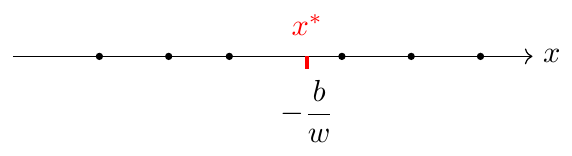
1D (\,\(\mathbb{R}\)\,) -- a point
In one dimension ($d=1$) the hyperplane is a single point. With $w\neq0$ and scalar $x$, \[ w x + b = 0 \qquad\Longrightarrow\qquad x = -\frac{b}{w}. \]
2D (\,\(\mathbb{R}^2\)\,) -- a line
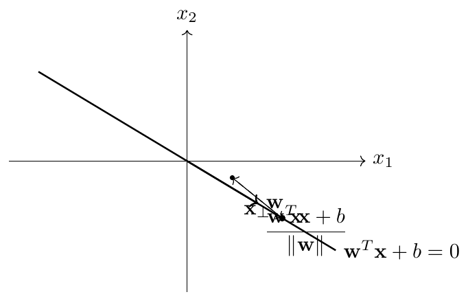
In two dimensions the hyperplane is a line. For $\mathbf{x}=(x_1,x_2)^T$ and $\mathbf{w}=(w_1,w_2)^T$: \[ w_1 x_1 + w_2 x_2 + b = 0. \] The signed (orthogonal) distance from a point $\mathbf{x}$ to the line is \[ \mathrm{dist}(\mathbf{x},H)=\frac{\mathbf{w}^T\mathbf{x}+b}{\|\mathbf{w}\|}. \]
General $d$ (\,\(\mathbb{R}^d\)\,) -- derivation (orthogonal projection)
Take any $\mathbf{x}\in\mathbb{R}^d$. Decompose $\mathbf{x}$ into a point on the hyperplane $ \mathbf{x}_H\in H$ plus a component parallel to $\mathbf{w}$: \[ \mathbf{x} = \mathbf{x}_H + t\frac{\mathbf{w}}{\|\mathbf{w}\|},\qquad t\in\mathbb{R}. \] Because $\mathbf{x}_H$ satisfies $\mathbf{w}^T\mathbf{x}_H+b=0$, substitute into that relation: \[ 0=\mathbf{w}^T\mathbf{x}_H+b =\mathbf{w}^T\!\Big(\mathbf{x}-t\frac{\mathbf{w}}{\|\mathbf{w}\|}\Big)+b =\mathbf{w}^T\mathbf{x}-t\|\mathbf{w}\|+b. \] Solve for $t$ to obtain the signed orthogonal distance from $\mathbf{x}$ to $H$: \[ \boxed{\;t=\frac{\mathbf{w}^T\mathbf{x}+b}{\|\mathbf{w}\|}\; }. \] Hence $\mathbf{w}^T\mathbf{x}+b$ is proportional to the signed distance (scale factor $\|\mathbf{w}\|$).
Decision function (linear classifier)
The linear decision function used in SVM and other linear classifiers is \[ f(\mathbf{x})=\mathbf{w}^T\mathbf{x}+b, \] and the class prediction is $\hat y=\operatorname{sign}(f(\mathbf{x}))$. \[ \boxed{\,y=\mathbf{w}^T\mathbf{x}+b\,} \]
Hard-Margin SVM: geometry, formulation and solution
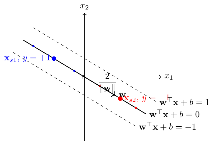
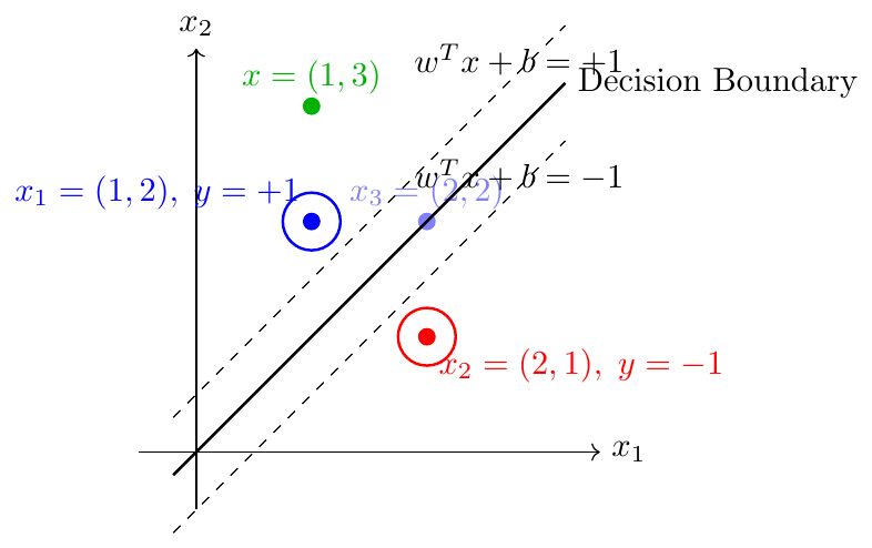
Geometric figure and support vectors (2D)
Concept (informal)
The maximal margin classifier chooses the separating hyperplane so that the perpendicular distance between the two parallel margin hyperplanes \[ \mathbf{w}^\top\mathbf{x}+b=+1\quad\text{and}\quad\mathbf{w}^\top\mathbf{x}+b=-1 \] is maximized. Points lying exactly on these margins are the support vectors; they alone determine the classifier.
Derivation of the optimization problem
Distance between margin planes = $2/\|\mathbf{w}\|$. Maximizing this is equivalent to minimizing $\|\mathbf{w}\|^2$ subject to correct classification with margin: \[ y_i(\mathbf{w}^\top\mathbf{x}_i + b)\ge 1,\qquad i=1,\dots,n. \] Thus the primal problem (hard margin) is \[ \boxed{\;\min_{\mathbf{w},b}\; \frac{1}{2}\|\mathbf{w}\|^2 \quad\text{s.t.}\quad y_i(\mathbf{w}^\top\mathbf{x}_i + b)\ge 1\; (i=1,\dots,n).\;} \]
Lagrangian, KKT and consequence
Form Lagrangian with multipliers $\alpha_i\ge0$: \[ \mathcal{L}(\mathbf{w},b,\boldsymbol{\alpha}) =\tfrac{1}{2}\|\mathbf{w}\|^2 - \sum_{i=1}^n\alpha_i\big(y_i(\mathbf{w}^\top\mathbf{x}_i+b)-1\big). \] Stationarity conditions (set partial derivatives to zero) give \[ \frac{\partial\mathcal{L}}{\partial\mathbf{w}}=0 \;\Rightarrow\; \boxed{\;\mathbf{w}=\sum_{i=1}^n \alpha_i y_i \mathbf{x}_i\;},\qquad \frac{\partial\mathcal{L}}{\partial b}=0 \;\Rightarrow\; \sum_{i=1}^n \alpha_i y_i = 0. \] Complementary slackness states that for each $i$ either $\alpha_i=0$ (non-support) or \[ y_i(\mathbf{w}^\top\mathbf{x}_i+b)=1 \quad\text{(support vector)}. \] Hence support vectors are exactly those with $\alpha_i>0$.
Dual statement (brief) and solution strategy
The dual quadratic program is \[ \begin{aligned} &\max_{\boldsymbol{\alpha}}\; \sum_{i=1}^n\alpha_i - \tfrac{1}{2}\sum_{i,j}\alpha_i\alpha_j y_i y_j \mathbf{x}_i^\top\mathbf{x}_j,\\ &\text{subject to }\; \alpha_i\ge0,\;\; \sum_{i=1}^n\alpha_i y_i=0. \end{aligned} \] Solve for $\alpha^*$ (QP). Recover primal weight using the boxed formula above.
Bias $b$ (practical formula)
For any support vector $s$ (with $\alpha_s>0$) we have equality: \[ y_s(\mathbf{w}^\top\mathbf{x}_s+b)=1 \;\Rightarrow\; \boxed{\;b = y_s - \mathbf{w}^\top\mathbf{x}_s\; }. \] In practice average over all support vectors to get a numerically stable $b$: \[ b \;=\; \frac{1}{|S|}\sum_{s\in S}\big(y_s-\mathbf{w}^\top\mathbf{x}_s\big),\qquad S=\{i:\alpha_i>0\}. \]
Summary (final formulas)
\[ \boxed{\,\mathbf{w}=\sum_{i=1}^n \alpha_i^* y_i \mathbf{x}_i\,,\qquad b=\text{average}_{s\in S}\big(y_s-\mathbf{w}^\top\mathbf{x}_s\big)\,} \] Support vectors are those indices with $\alpha_i^*>0$ and they alone define the classifier. Classifier function \[ f(\mathbf{x})=\operatorname{sign}(\mathbf{w}^\top \mathbf{x}+b). \]
Training data and Lagrange multipliers: \[ \begin{array}{c|c|c|c} i & \mathbf{x}_i & y_i & \alpha_i\\\hline 1 & (1,2) & +1 & 2\\ 2 & (2,1) & -1 & 2\\ 3 & (2,2) & +1 & 0 \end{array} \qquad\text{Classify }\mathbf{x}=(1,3). \]
Step 1 — Compute weight vector \(\mathbf{w}\) Use the relation \(\mathbf{w}=\sum_{i}\alpha_i y_i \mathbf{x}_i\). Compute each term explicitly:
\[ \begin{aligned} \alpha_1 y_1 \mathbf{x}_1 &= 2\cdot(+1)\cdot\begin{pmatrix}1\\2\end{pmatrix} = \begin{pmatrix}2\\4\end{pmatrix},\\[4pt] \alpha_2 y_2 \mathbf{x}_2 &= 2\cdot(-1)\cdot\begin{pmatrix}2\\1\end{pmatrix} = \begin{pmatrix}-4\\-2\end{pmatrix},\\[4pt] \alpha_3 y_3 \mathbf{x}_3 &= 0\cdot(+1)\cdot\begin{pmatrix}2\\2\end{pmatrix} = \begin{pmatrix}0\\0\end{pmatrix}. \end{aligned} \]
Sum the terms: \[ \mathbf{w} = \begin{pmatrix}2\\4\end{pmatrix} + \begin{pmatrix}-4\\-2\end{pmatrix} + \begin{pmatrix}0\\0\end{pmatrix} = \begin{pmatrix}-2\\2\end{pmatrix}. \]
Step 2 — Compute bias \(b\) For any support vector \(s\) with \(\alpha_s>0\) we have \[ y_s(\mathbf{w}^\top\mathbf{x}_s + b)=1 \quad\Longrightarrow\quad b = y_s - \mathbf{w}^\top\mathbf{x}_s. \] Support vectors here are indices \(1\) and \(2\) (since \(\alpha_1=2,\;\alpha_2=2,\;\alpha_3=0\)).
Compute \(\mathbf{w}^\top\mathbf{x}_1\): \[ \mathbf{w}^\top\mathbf{x}_1 = (-2)\cdot 1 + 2\cdot 2 = -2 + 4 = 2. \quad\Rightarrow\quad b_1 = y_1 - \mathbf{w}^\top\mathbf{x}_1 = 1 - 2 = -1. \]
Compute \(\mathbf{w}^\top\mathbf{x}_2\): \[ \mathbf{w}^\top\mathbf{x}_2 = (-2)\cdot 2 + 2\cdot 1 = -4 + 2 = -2. \quad\Rightarrow\quad b_2 = y_2 - \mathbf{w}^\top\mathbf{x}_2 = -1 -(-2) = -1 + 2 = 1. \]
Average the two values for numerical stability: \[ b = \frac{b_1 + b_2}{2} = \frac{-1 + 1}{2} = 0. \]
(Using a single support vector would give \(b=-1\) or \(b=1\); averaging is standard practice.)
Step 3 — Decision function for \(\mathbf{x}=(1,3)\) Compute the raw decision value \(f(\mathbf{x})=\mathbf{w}^\top\mathbf{x}+b\).
First the dot product: \[ \mathbf{w}^\top\mathbf{x} = (-2)\cdot 1 + 2\cdot 3 = -2 + 6 = 4. \] Add \(b=0\): \[ f(1,3) = 4 + 0 = 4. \]
Step 4 — Classification (sign rule) Apply \(\hat y = \operatorname{sign}(f(\mathbf{x}))\): \[ \operatorname{sign}(4) = +1. \]
Remarks Support vectors are indices \(1\) and \(2\) (those with \(\alpha_i>0\)). The classifier parameters are \[ \mathbf{w} = \begin{pmatrix}-2\\2\end{pmatrix},\qquad b=0. \]
Soft Margin - Support Vector Classifier
Motivation: why soft margin
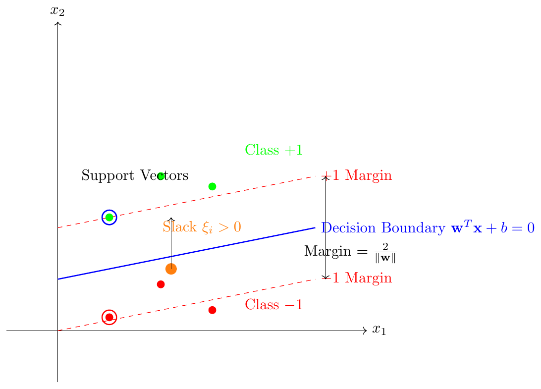
The hard-margin SVM requires exact linear separability of the training data. In practice this is brittle: outliers, mislabels and naturally overlapping classes make the hard-margin program infeasible or lead to poor generalization. The soft-margin SVM remedies this by introducing nonnegative slack variables $\xi_i\ge0$ which permit controlled violations of the margin constraint. The total violation is penalized in the objective with weight $C>0$, which controls the trade-off between model complexity (large margin) and training error.
Primal formulation (soft margin)
Given labeled data $\{(\mathbf{x}_i,y_i)\}_{i=1}^n$ with $y_i\in\{\pm1\}$, the soft-margin primal optimization problem is: \[ \begin{aligned} &\min_{\mathbf{w},\,b,\,\boldsymbol{\xi}}\quad \frac{1}{2}\|\mathbf{w}\|^2 + C\sum_{i=1}^n \xi_i,\\[4pt] &\text{subject to}\qquad y_i\big(\mathbf{w}^\top\mathbf{x}_i + b\big) \ge 1 - \xi_i,\qquad \xi_i \ge 0,\qquad i=1,\dots,n. \end{aligned} \] The hyperparameter $C>0$ trades off margin size against penalty for margin violations.
Lagrangian and stationarity
Introduce Lagrange multipliers $\alpha_i\ge0$ for the margin constraints and $\mu_i\ge0$ for $\xi_i\ge0$. The Lagrangian is \[ \mathcal{L}(\mathbf{w},b,\boldsymbol{\xi},\boldsymbol{\alpha},\boldsymbol{\mu}) = \tfrac12\|\mathbf{w}\|^2 + C\sum_{i=1}^n\xi_i - \sum_{i=1}^n \alpha_i\big(y_i(\mathbf{w}^\top\mathbf{x}_i+b)-1+\xi_i\big) - \sum_{i=1}^n \mu_i \xi_i. \] Stationarity conditions (set partial derivatives to zero) yield: \[ \frac{\partial\mathcal{L}}{\partial\mathbf{w}}=0 \ \Rightarrow\ \mathbf{w}=\sum_{i=1}^n \alpha_i y_i \mathbf{x}_i, \] \[ \frac{\partial\mathcal{L}}{\partial b}=0 \ \Rightarrow\ \sum_{i=1}^n \alpha_i y_i = 0, \] \[ \frac{\partial\mathcal{L}}{\partial\xi_i}=0 \ \Rightarrow\ C-\alpha_i-\mu_i = 0 \ \Rightarrow\ 0\le\alpha_i\le C. \]
Dual problem
Eliminating $\mathbf{w}$ and $b$ leads to the dual quadratic program \[ \begin{aligned} &\max_{\boldsymbol{\alpha}} \quad \sum_{i=1}^n \alpha_i \;-\; \tfrac12\sum_{i,j=1}^n \alpha_i\alpha_j y_i y_j \mathbf{x}_i^\top\mathbf{x}_j,\\[4pt] &\text{subject to}\quad 0 \le \alpha_i \le C,\quad \sum_{i=1}^n \alpha_i y_i = 0. \end{aligned} \] This dual is a concave quadratic program in the variables $\alpha_i$ with simple bound constraints and one linear equality.
KKT conditions and practical consequences
From complementary slackness and stationarity we derive the operational rules:
Primal-dual relation (weights): \[ \boxed{\ \mathbf{w}=\sum_{i=1}^n \alpha_i y_i \mathbf{x}_i\ }\quad\text{(always).} \]
Dual feasibility: $0\le\alpha_i\le C$ for every $i$, and $\sum_i\alpha_i y_i = 0$.
Complementary slackness (margin constraint): \[ \alpha_i\big(y_i(\mathbf{w}^\top\mathbf{x}_i+b)-1+\xi_i\big)=0. \] Thus:
If $\alpha_i=0$, then the margin constraint may be slack (point lies strictly outside margin) and we have $y_i(\mathbf{w}^\top\mathbf{x}_i+b)>1$ and $\xi_i=0$.
If $0<\alpha_i<C$, then necessarily $\xi_i=0$ and $y_i(\mathbf{w}^\top\mathbf{x}_i+b)=1$ (the point lies exactly on the margin boundary) — these are support vectors on the margin.
If $\alpha_i=C$, then $\mu_i=0$ and $\xi_i$ may be $>0$; complementary slackness for $\alpha_i$ enforces \[ y_i(\mathbf{w}^\top\mathbf{x}_i+b)=1-\xi_i \le 1, \] so such points lie inside the margin (or are misclassified).
Stationarity wrt $\xi_i$: $C-\alpha_i-\mu_i=0$ together with $\mu_i\xi_i=0$ implies:
If $\alpha_i<C$ then $\mu_i>0$ and therefore $\xi_i=0$.
If $\alpha_i=C$ then $\mu_i=0$ and $\xi_i$ may be $>0$.
Bias $b$: For any $i$ with $0<\alpha_i<C$ (i.e. a margin support vector) we have the exact identity \[ \boxed{\ b = y_i - \mathbf{w}^\top\mathbf{x}_i\ }. \] In practice average $b$ over all indices with $0<\alpha_i<C$ to increase numerical stability.
Summary table: \(\alpha_i\), \(\xi_i\) and geometric meaning

Consider the training set and parameter: \[ \begin{array}{c|c|c|c} i & \mathbf{x}_i & y_i & \alpha_i \\\hline 1 & (1,\,0) & +1 & 0.30 \\ 2 & (-1,\,0) & -1 & 0.60 \\ 3 & (0,\,0) & +1 & 0.10 \end{array} \qquad C = 0.6. \]
Given the supplied vector \[ \boldsymbol{\alpha} = (0.30,\;0.60,\;0.10), \qquad y = (+1,\;-1,\;+1), \] compute the primal weight vector \[ \mathbf{w}=\sum_{i=1}^3 \alpha_i y_i \mathbf{x}_i. \]
\[ \begin{aligned} \alpha_1 y_1 \mathbf{x}_1 &= 0.30\cdot(+1)\cdot(1,0) = (0.30,\,0),\\[6pt] \alpha_2 y_2 \mathbf{x}_2 &= 0.60\cdot(-1)\cdot(-1,0) = 0.60\cdot(1,0) = (0.60,\,0),\\[6pt] \alpha_3 y_3 \mathbf{x}_3 &= 0.10\cdot(+1)\cdot(0,0) = (0,0). \end{aligned} \]
\[ \boxed{\;\mathbf{w} = (0.30+0.60,\,0) = (0.90,\,0)\; }. \]
Per-support bias values (KKT equality for $0<\alpha_i<C$) For any index with $0<\alpha_i<C$ the KKT equality gives \[ y_i(\mathbf{w}^\top\mathbf{x}_i + b) = 1 \quad\Longrightarrow\quad b = y_i - \mathbf{w}^\top\mathbf{x}_i. \]
Apply to the two non-bound support indices $i=1$ and $i=3$: \[ \begin{aligned} b_1 &= 1 - (0.90,0)\cdot(1,0) = 1 - 0.90 = 0.10,\\[6pt] b_3 &= 1 - (0.90,0)\cdot(0,0) = 1 - 0 = 1.00. \end{aligned} \]
Practical (heuristic) averaging of these two values yields \[ \boxed{\;b = \frac{b_1 + b_3}{2} = \frac{0.10 + 1.00}{2} = 0.55\; }. \]
Classification of $\mathbf{x}=(1,3)$ with the chosen $(\mathbf{w},b)$ Decision function: \[ f(\mathbf{x}) = \operatorname{sign}(\mathbf{w}^\top\mathbf{x} + b). \] Compute: \[ \mathbf{w}^\top(1,3) + b = (0.90,0)\cdot(1,3) + 0.55 = 0.90 + 0 + 0.55 = 1.45, \] hence \[ \boxed{\,f(1,3) = \operatorname{sign}(1.45) = +1\,.} \]
Hinge Loss
In Soft Margin SVM, not all violations are treated equally. The classifier applies a penalty that increases as a point moves deeper into the margin or crosses the decision boundary. This behaviour is visually described by the hinge loss curve.
Conceptual interpretation:
Correct and confidently classified points incur zero penalty.
Points inside the margin incur a gradual linear penalty.
Misclassified points incur the highest penalty.
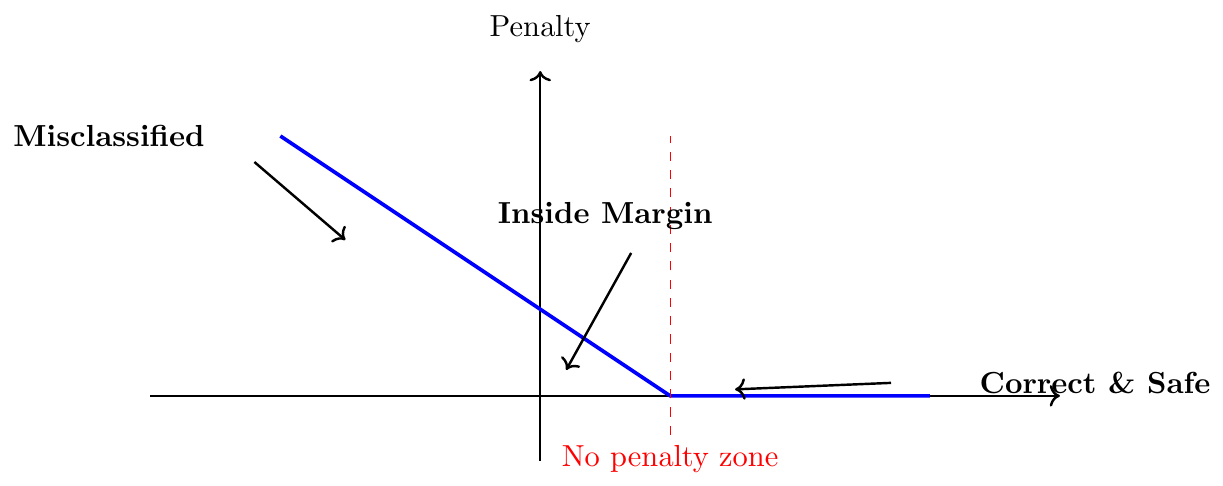
Figure Interpretation:
The slanted segment (slope =1) represents increasing penalty for margin violations.
The flat segment (slope =0) represents regions where points are sufficiently confident and incur no cost.
The hinge point marks the transition between penalized and unpenalized zones.
This illustrates how Soft Margin SVM balances classification accuracy and robustness by tolerating controlled violations rather than enforcing strict separability.
Kernel Trick
Linear SVM works by finding a hyperplane that separates classes. However, real-world data is often non-linear, as shown below:
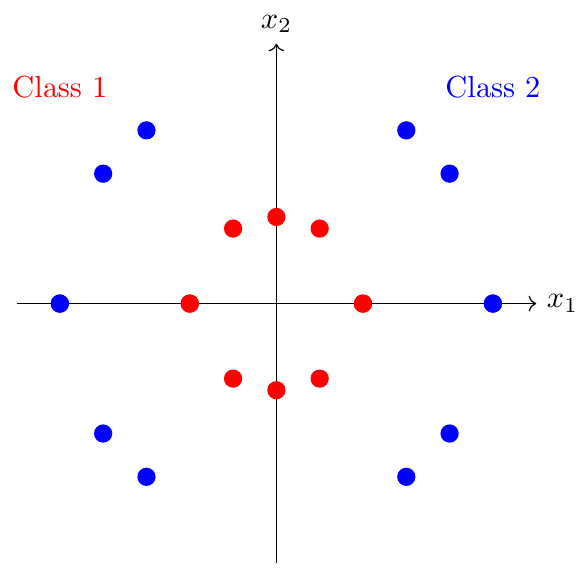
Clearly, no straight line can separate these classes. We need a non-linear mapping.
Feature Mapping $\phi(\cdot)$
The idea is to map input features to a higher-dimensional space where data becomes linearly separable:
\[ \phi: \mathbb{R}^n \to \mathbb{R}^m, \quad m>n \]
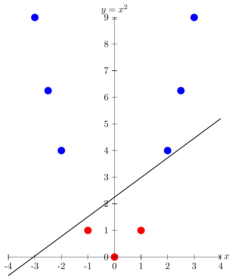
A function $\phi(x)$ transforms input $x$ to a higher-dimensional space to make the data linearly separable.
Example: 1D to 2D Mapping
Consider 1D data $x \in \mathbb{R}$ and map it to 2D using:
\[ \phi(x) = (x, x^2) \]

Kernel Function
Instead of computing $\phi(x)$ explicitly, we use a kernel function:
\[ K(x_i, x_j) = \phi(x_i) \cdot \phi(x_j) \]
A kernel function computes the dot product of two vectors in the higher-dimensional space without explicitly computing the mapping $\phi(x)$.
The ``Trick'' with Dot Products
We can write the SVM classifier as:
\[ f(x) = \sum_{i=1}^{N} \alpha_i y_i K(x_i, x) + b \]
Here, $K(x_i,x)$ implicitly uses the higher-dimensional mapping. This avoids costly computations in high-dimensional space.
Common Kernel Functions
Linear Kernel: $K(x_i,x_j) = x_i \cdot x_j$
Polynomial Kernel: $K(x_i,x_j) = (x_i \cdot x_j + c)^d$
RBF / Gaussian Kernel: $K(x_i,x_j) = \exp\Big(-\frac{\|x_i-x_j\|^2}{2\sigma^2}\Big)$
Sigmoid Kernel: $K(x_i,x_j) = \tanh(\kappa x_i \cdot x_j + c)$
The kernel trick allows SVM to perform non-linear classification efficiently by:
Mapping data to higher dimensions via $\phi(x)$
Using kernel functions $K(x_i,x_j)$ to compute dot products
Avoiding explicit computation in high-dimensional space
Neural Network Models
Feed-Forward Neural Networks (FFNN)
Network Architecture and Notation
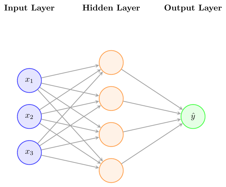
A Feed-Forward Neural Network (FFNN) is a computational model inspired by the biological neuron. It consists of multiple layers of interconnected nodes (neurons), where information flows in one direction — from input to output — without any feedback loops.
Notation:
$x_i$ : Input features ($i = 1, 2, \dots, d$)
$w_{ij}^{(l)}$ : Weight connecting neuron $j$ in layer $(l-1)$ to neuron $i$ in layer $(l)$
$b_i^{(l)}$ : Bias term for neuron $i$ in layer $(l)$
$a_i^{(l)}$ : Activation (output) of neuron $i$ in layer $(l)$
—
Activation Functions (Sigmoid, ReLU, Tanh)
The activation function introduces non-linearity, allowing the network to model complex relationships.
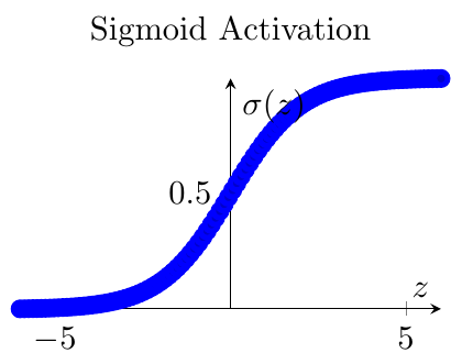
1. Sigmoid Function: \[ \sigma(z) = \frac{1}{1 + e^{-z}} \]
It maps input values to $(0,1)$, useful for probabilities.
2. Tanh Function: \[ \tanh(z) = \frac{e^z - e^{-z}}{e^z + e^{-z}} \] Range: $(-1,1)$ — centered around zero.
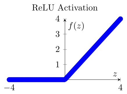
3. ReLU (Rectified Linear Unit): \[ f(z) = \max(0, z) \] It is widely used due to faster convergence and less vanishing gradient.
—
Forward Propagation and Loss Computation
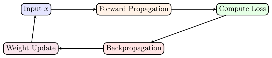
In forward propagation, data moves from the input layer through hidden layers to produce the output.
For a single neuron: \[ z_i^{(l)} = \sum_{j} w_{ij}^{(l)} a_j^{(l-1)} + b_i^{(l)} \] \[ a_i^{(l)} = f(z_i^{(l)}) \]
For the output layer in regression: \[ \hat{y} = a^{(L)} = f(z^{(L)}) \]
Example: Suppose input $x = [1, 2]$, weights $w = [0.5, -1]$, bias $b = 0.2$ and $f(z) = \text{ReLU}(z)$.
\[ z = (1)(0.5) + (2)(-1) + 0.2 = -1.3 \implies a = 0 \]
So the neuron output is $0$.
Loss Function (Mean Squared Error): \[ L = \frac{1}{N} \sum_{i=1}^N (y_i - \hat{y}_i)^2 \]
—
Backpropagation Algorithm and Gradient Flow
Goal: Adjust weights $w$ and biases $b$ to minimize the loss.
\[ w_{ij}^{(l)} \leftarrow w_{ij}^{(l)} - \eta \frac{\partial L}{\partial w_{ij}^{(l)}} \] where $\eta$ is the learning rate.
Gradient computation: \[ \frac{\partial L}{\partial w_{ij}^{(l)}} = \delta_i^{(l)} a_j^{(l-1)} \] \[ \delta_i^{(l)} = f'(z_i^{(l)}) \sum_k \delta_k^{(l+1)} w_{ki}^{(l+1)} \]
—
Vanishing/Exploding Gradient Problem
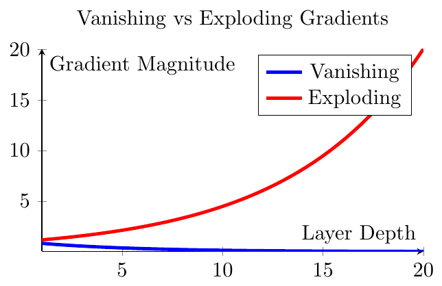
Definition: When gradients become extremely small (vanish) or large (explode) during backpropagation, training becomes unstable.
Why it happens: \[ \delta^{(l)} = f'(z^{(l)}) W^{(l+1)T} \delta^{(l+1)} \] If $|f'(z^{(l)})| < 1$ repeatedly (e.g., Sigmoid), gradients shrink exponentially → vanishing. If weights $> 1$, gradients may explode.
Remedies:
Use ReLU instead of Sigmoid or Tanh.
Normalize inputs and use Batch Normalization.
Use residual connections (as in ResNet).
Initialize weights carefully (e.g., Xavier or He initialization).
—
FFNN learns a non-linear mapping from inputs to outputs via multiple layers.
Activation functions enable non-linearity.
Forward pass computes prediction; backward pass updates weights.
Deep networks suffer from vanishing/exploding gradients, which can be mitigated by normalization and better initialization.
Multi-Layer Perceptron (MLP)
Universal Approximation Theorem (Conceptual Insight)
The Universal Approximation Theorem states that a feed-forward neural network with:
at least one hidden layer,
finite number of neurons,
and a non-linear activation function (e.g., sigmoid, ReLU, tanh)
can approximate any continuous function $f: \mathbb{R}^n \to \mathbb{R}$ to an arbitrary degree of accuracy given sufficient neurons.
Reasoning: Hidden layers provide non-linear transformations, allowing the network to capture complex mappings between inputs and outputs that linear models cannot. This theorem gives theoretical assurance of MLP's capability, although practical training may require regularization and careful weight initialization.
Suppose we want to approximate $f(x) = \sin(x)$ over $[0, \pi]$.
Using a single hidden layer with 10 neurons and a sigmoid activation, an MLP can approximate $\sin(x)$ closely.
Increasing neurons improves accuracy but may increase overfitting risk.
Training and Regularization Techniques
Training involves minimizing a loss function (e.g., MSE for regression, cross-entropy for classification) using:
Forward propagation to compute outputs.
Backpropagation to compute gradients w.r.t weights.
Gradient-based optimization (e.g., SGD, Adam) to update weights.
To prevent overfitting:
L2 Regularization (Weight Decay): Adds $\lambda \sum w^2$ to loss.
Dropout: Randomly zeroes a fraction of hidden neurons during training.
Early Stopping: Halt training when validation loss stops improving.
A classification MLP with 3 hidden layers (64, 32, 16 neurons) overfits training data. Applying dropout of 0.3 and L2 regularization $\lambda = 0.01$ improves validation accuracy by 8%.
Comparison with Traditional ML Models
Linear Models: Can only capture linear relationships.
Decision Trees: Non-linear, but may struggle with high-dimensional data and interactions.
MLPs: Capture complex non-linear patterns and interactions, scalable with more data.
Predicting housing prices:
Linear regression underfits the data due to non-linear interactions.
Random Forest captures some non-linearities but saturates at 90% R-squared.
MLP with 2 hidden layers achieves 97% R-squared by modeling complex interactions.
Advantages and Limitations of MLPs
Can approximate any continuous function (Universal Approximation).
Flexible architecture (number of layers/neurons).
Suitable for regression, classification, and complex pattern recognition.
Requires large amounts of labeled data.
Computationally intensive, especially with many layers.
Prone to overfitting without proper regularization.
Difficult to interpret compared to simple models.
A small dataset (500 samples, 10 features) trained with a deep MLP (5 hidden layers) overfits drastically. Using a shallow MLP (2 hidden layers) with dropout maintains similar accuracy but improves generalization.