Model Evaluation and Generalization
Cross-Validation Methods
Cross-validation is a statistical method used to estimate the performance of machine learning models on unseen data. It is widely used for model evaluation and hyperparameter tuning, especially when the dataset is limited.
Hold-Out Validation
Concept: Hold-out validation splits the dataset into two disjoint subsets:
Training set: used to fit the model.
Test set: used to evaluate the model performance.
Procedure:
Randomly split the data, e.g., 70% training and 30% test.
Train the model on the training set.
Compute evaluation metrics (MSE, accuracy, etc.) on the test set.
Advantages: Simple, fast. Disadvantages: Sensitive to the random split, may not utilize all data for training.

Leave-One-Out (LOO) Cross-Validation
Concept: LOO is an extreme case of k-fold cross-validation where $k=n$ (number of samples). Each sample is used once as a test set, and the model is trained on the remaining $n-1$ samples.
Procedure:
For each sample $i=1,\dots,n$, train the model on all other samples except $i$.
Test the model on the excluded sample.
Average the evaluation metrics across all iterations.
Advantages: Uses maximum data for training, low bias. Disadvantages: Computationally expensive for large datasets.
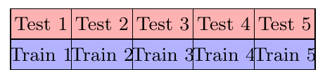
k-Fold Cross-Validation
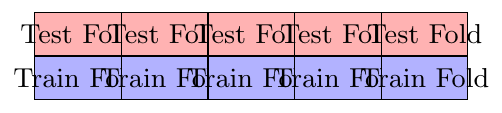
Concept: In k-fold cross-validation, the dataset is divided into $k$ roughly equal folds. Each fold is used once as a test set, and the remaining $k-1$ folds are used for training.
Procedure:
Split the dataset into $k$ folds.
For $i=1$ to $k$, train on $k-1$ folds and test on the $i$-th fold.
Average the evaluation metrics over all folds.
Advantages: Reduces variance of the performance estimate, uses all data for training and testing. Choice of $k$: $k=5$ or $10$ are commonly used.
Model Selection and Hyperparameter Tuning
Concept: Cross-validation is extensively used to select the best model or hyperparameters, e.g., regularization strength, number of neighbors ($k$ in k-NN), or depth of decision trees.
Procedure:
Define a grid of hyperparameter values.
For each combination, perform k-fold CV.
Select the combination with the best average performance.
Reasoning: Using cross-validation prevents overfitting on a single validation set and provides a more robust estimate of model performance.
Examples: Cross-Validation Methods
Hold-Out Validation Example: House Prices
A dataset contains 50 samples of house prices with features: area, bedrooms, age. We split it 70% training and 30% test. Train a linear regression model and evaluate MSE on the test set: MSE = 25.
Interpretation: Hold-out validation gives an estimate of test error. The result may vary if the random split changes.
Leave-One-Out Cross-Validation Example
Dataset: $X = [1,2,3,4]$, $Y = [2,3,2.5,5]$.
Perform LOO CV for linear regression:
Iteration 1: Train on $\{2,3,4\}$, test on 1 → Predicted $\hat{Y}_1 = 2.1$, squared error = 0.01
Iteration 2: Train on $\{1,3,4\}$, test on 2 → Predicted $\hat{Y}_2 = 2.9$, squared error = 0.01
Iteration 3: Train on $\{1,2,4\}$, test on 3 → Predicted $\hat{Y}_3 = 2.7$, squared error = 0.04
Iteration 4: Train on $\{1,2,3\}$, test on 4 → Predicted $\hat{Y}_4 = 4.8$, squared error = 0.04
LOO CV error: $CV_{LOO} = \frac{0.01+0.01+0.04+0.04}{4} = 0.025$
k-Fold Cross-Validation Example
Dataset: 12 samples. Perform 4-fold CV for a k-NN model ($k=3$):
Split dataset into 4 folds of 3 samples each.
Iteration 1: Train on folds 2-4, test fold 1 → accuracy = 0.67
Iteration 2: Train on folds 1,3,4, test fold 2 → accuracy = 0.67
Iteration 3: Train on folds 1,2,4, test fold 3 → accuracy = 1.0
Iteration 4: Train on folds 1-3, test fold 4 → accuracy = 0.67
4-fold CV accuracy: $\frac{0.67+0.67+1.0+0.67}{4} = 0.7525$
Hyperparameter Tuning using k-Fold CV
We want to choose $k$ in k-NN for a dataset of 100 samples. Test $k = 1,3,5,7$ using 5-fold CV:
$k=1$: average accuracy = 0.78
$k=3$: average accuracy = 0.82
$k=5$: average accuracy = 0.81
$k=7$: average accuracy = 0.79
Best choice: $k=3$ because it gives the highest cross-validation accuracy.
Interpretation: k-fold CV helps select hyperparameters while avoiding overfitting.
LOO vs Hold-Out Comparison
Dataset: 10 samples for linear regression.
Hold-Out: Train 7, Test 3 → test MSE = 10.5
LOO: Compute prediction for each sample leaving it out → average MSE = 9.8
Observation: LOO provides a more stable estimate because it uses almost all data for training, whereas hold-out can vary depending on the random split. However, LOO is more computationally expensive.
ROC & AUC
The ROC curve (Receiver Operating Characteristic curve) is a standard way to visualize and evaluate the performance of a binary classifier across all possible decision thresholds. The curve plots the True Positive Rate (TPR) on the vertical axis against the False Positive Rate (FPR) on the horizontal axis. The AUC (Area Under the ROC Curve) is a single scalar summarizing the ROC; it ranges from 0 to 1. Higher AUC indicates better ability to separate positive and negative classes.
Confusion matrix and rates
A confusion matrix for a binary classifier:
\[ \begin{array}{c|cc} & \text{Predicted Positive} & \text{Predicted Negative} \\ \hline \text{Actual Positive} & \mathrm{TP} & \mathrm{FN} \\ \text{Actual Negative} & \mathrm{FP} & \mathrm{TN} \end{array} \]
From this we define: \[ \mathrm{TPR} \;=\; \frac{\mathrm{TP}}{\mathrm{TP}+\mathrm{FN}} \qquad\text{(True Positive Rate, a.k.a. Recall)} \] \[ \mathrm{FPR} \;=\; \frac{\mathrm{FP}}{\mathrm{FP}+\mathrm{TN}} \qquad\text{(False Positive Rate, a.k.a. False alarm rate)} \]
What is a decision threshold?
A probabilistic classifier outputs a score \(s(x)\in[0,1]\). To obtain labels we pick a threshold \(\tau\) and predict positive if \(s(x)\ge\tau\). Different choices of \(\tau\) produce different confusion matrices and thus different (TPR,FPR) pairs. The ROC curve collects those pairs for all thresholds.
ROC curve and AUC (intuition)
Each point on the ROC corresponds to a threshold and shows the trade-off between detection rate (TPR) and false-alarm rate (FPR).
The AUC is the area under the ROC curve. It has the following useful interpretation: \[ \mathrm{AUC} = P\big(s(X_+) > s(X_-)\big) \quad\text{(probability a random positive ranks above a random negative).} \]
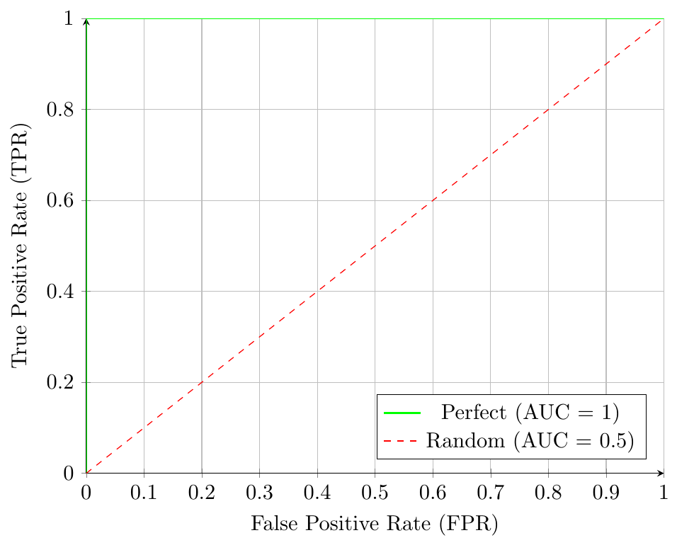
Values: AUC = 1.0 (perfect ranking), AUC = 0.5 (random), AUC < 0.5 (means ranking reversed).
Worked numeric example (spam detector)
We reuse the concrete threshold outcomes described earlier (counts are not all given; we present the rates you provided):
At three decision thresholds we observed:
\[ \begin{array}{l|c|c} \text{Threshold} & \mathrm{TPR}=\dfrac{\text{TP}}{\text{TP}+\text{FN}} & \mathrm{FPR}=\dfrac{\text{FP}}{\text{FP}+\text{TN}} \\ \hline 0.50 & 800/(800+100)=0.89 & 500/(500+8600)=0.06 \\ 0.80 & 600/(600+300)=0.67 & 100/(100+9000)=0.01 \\ 0.95 & 200/(200+700)=0.22 & 10/(10+9090)=0.001 \end{array} \]
Interpretation:
At \(\tau=0.50\) the detector is lenient: high recall (0.89) but more false alarms (FPR=0.06).
At \(\tau=0.95\) the detector is strict: low recall (0.22) and almost no false alarms (FPR=0.001).
Plotting the ROC curve (from these points)
To draw the ROC we plot the FPR on the \(x\)-axis and TPR on the \(y\)-axis for each threshold and connect the points (also include \((0,0)\) and \((1,1)\)).
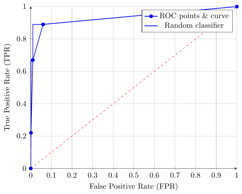
Note: the curve above is drawn from the listed (FPR,TPR) pairs; with more threshold values the curve becomes smoother.
Computing AUC (brief)
A common numerical method is the trapezoidal rule on the ROC points ordered by FPR: \[ \mathrm{AUC} \approx \sum_{i} (x_{i+1}-x_i)\,\frac{y_i+y_{i+1}}{2}, \] where \(x_i\) are FPRs and \(y_i\) are the corresponding TPRs. Use sufficiently many thresholds for a good estimate.
Perfect and random classifiers (illustration)
Practical notes
AUC is threshold-independent: it summarizes ranking quality for all thresholds.
Use-case sensitivity: if the positive class is rare, Precision–Recall curves may be more informative than ROC.
Interpretation: AUC $=0.5$ means no discrimination (random), AUC close to 1.0 means excellent discrimination.
Choice of threshold: AUC does not choose a threshold — select \(\tau\) based on application-specific trade-offs (costs of FP vs FN).
Conclusion
ROC visualizes the trade-off between detecting positives and producing false alarms as the decision threshold varies. AUC condenses this visualization into a single number expressing the classifier's overall ranking ability.
Bias--Variance Trade-off
Understanding the Trade-off
In supervised learning, our goal is to build a model that generalizes well to unseen data. The performance of a model on unseen data can be decomposed into three components: bias, variance, and irreducible error (noise).
\[ \text{Expected Test Error} = \text{Bias}^2 + \text{Variance} + \text{Irreducible Error} \]
Each term has an intuitive meaning:
Bias: Error due to simplifying assumptions made by the model.
Variance: Error due to sensitivity of the model to small fluctuations in training data.
Irreducible Error: Noise inherent in the data that no model can explain.
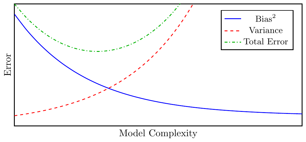
Figure: The bias–variance trade-off. As model complexity increases, bias decreases but variance increases. The total error is minimized at an optimal complexity.
Bias measures the error introduced by approximating a real-world problem (which may be extremely complex) by a simplified model. A high-bias model makes strong assumptions about the data and fails to capture important regularities.
\[ \text{Bias}^2 = [E(\hat{f}(x)) - f(x)]^2 \] Interpretation: It represents how far the average prediction of the model is from the true function $f(x)$.
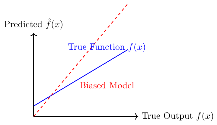
Figure: A biased model (red) systematically underestimates the true relationship (blue).
Variance measures how much the model’s predictions would vary if we trained it on different samples from the same population.
\[ \text{Var}[\hat{f}(x)] = E[(\hat{f}(x) - E[\hat{f}(x)])^2] \]
Interpretation: High-variance models fit training data too closely and perform poorly on unseen data. They have high sensitivity to random noise in the training set.
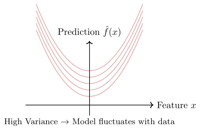
Figure: High-variance models change drastically with different data samples.
Increasing model complexity (e.g., higher polynomial degree) reduces bias but increases variance.
Decreasing model complexity increases bias but reduces variance.
The goal is to find the sweet spot minimizing total expected error.
Mathematical Derivation
Suppose $Y = f(X) + \varepsilon$, where $E[\varepsilon] = 0$, $\text{Var}(\varepsilon) = \sigma^2$. We predict $Y$ using an estimator $\hat{f}(X)$ obtained from data.
\[ E[(Y - \hat{f}(X))^2] = [E[\hat{f}(X)] - f(X)]^2 + E[(\hat{f}(X) - E[\hat{f}(X)])^2] + \sigma^2 \] \[ \Rightarrow \text{Expected Test MSE} = \underbrace{\text{Bias}^2}_{\text{Systematic Error}} + \underbrace{\text{Variance}}_{\text{Sensitivity to Data}} + \underbrace{\sigma^2}_{\text{Noise}} \]
—
Comparing Linear vs Polynomial Regression Models
Consider data generated from $Y = X^2 + \varepsilon$.
A linear regression model $Y = \beta_0 + \beta_1 X$ will have high bias (it cannot capture curvature).
A degree-10 polynomial will have low bias but very high variance.
Cross-validation typically identifies an intermediate degree (say, 3 or 4) that minimizes total test error.
—
Effect of Sample Size
When training a model on a small dataset:
Variance increases — the model depends heavily on limited data.
Bias may remain unchanged if model class is fixed.
Thus, increasing dataset size reduces variance but not bias.
—
High bias $\rightarrow$ underfitting (model too simple).
High variance $\rightarrow$ overfitting (model too complex).
Bias–variance trade-off can be visualized as an $U$-shaped total error curve.
Techniques like regularization (Ridge/Lasso) and cross-validation help control this trade-off.