Classification Models - I
Logistic Regression
Sigmoid Function and Log-Odds Interpretation
Logistic Regression is used when the dependent variable $Y$ is categorical (binary), i.e., it takes only two possible values — typically 0 or 1. It models the probability that $Y = 1$ as a function of input features $X_1, X_2, \dots, X_p$.
Unlike linear regression, where the output can take any real value, in classification we need outputs between 0 and 1, representing probabilities. Thus, the model uses the sigmoid (logistic) function to map real-valued predictions into the range $(0,1)$.
\[ p = P(Y = 1 \mid X) = \frac{1}{1 + e^{-z}} \] where $z = \beta_0 + \beta_1 X_1 + \beta_2 X_2 + \dots + \beta_p X_p$
$\sigma(z) = \frac{1}{1 + e^{-z}}$
$\sigma(z)$ is bounded between 0 and 1.
$\sigma'(z) = \sigma(z)(1 - \sigma(z))$ (important for gradient derivations)
Log-Odds Interpretation: The odds of an event are defined as $\dfrac{p}{1-p}$. Taking the logarithm gives the logit (log-odds):
\[ \log\left(\frac{p}{1-p}\right) = \beta_0 + \beta_1 X_1 + \beta_2 X_2 + \dots + \beta_p X_p \]
This means that logistic regression assumes the log-odds of the probability are linearly related to the predictors.
A model for disease prediction is: \[ \log\left(\frac{p}{1-p}\right) = -3 + 0.05 \times (\text{Age}) + 1.2 \times (\text{weight}) \] For a 40-year-old weight: \[ z = -3 + 0.05(40) + 1.2(1) = 0.2 \] \[ p = \frac{1}{1+e^{-0.2}} = 0.5498 \] Hence, the model predicts a 54.98% probability of having the disease.
Suppose $\beta_1 = 0.7$ for the predictor “Study Hours.” Then, increasing study hours by 1 increases the log-odds of passing by 0.7. In terms of odds: \[ e^{0.7} \approx 2.01 \] This means the odds of passing roughly double for each additional study hour.
Decision Boundary Analysis
The decision boundary separates predicted classes 0 and 1.
At boundary: $p = 0.5$
\[ \Rightarrow \frac{1}{1 + e^{-z}} = 0.5 \implies z = 0 \] \[ \beta_0 + \beta_1 X_1 + \beta_2 X_2 + \dots + \beta_p X_p = 0 \]
The decision boundary is linear in the input space for logistic regression. However, applying non-linear transformations to features (like polynomial terms) can produce non-linear boundaries.
For a 2D feature space: \[ z = -3 + 2x_1 + x_2 \] Decision boundary: \[ -3 + 2x_1 + x_2 = 0 \implies x_2 = 3 - 2x_1 \] This is a straight line dividing the classes.
If a polynomial term is added: \[ z = 1 + 0.5x_1^2 + x_2 \] Then, the decision boundary: \[ x_2 = -1 - 0.5x_1^2 \] is non-linear, showing the flexibility of logistic regression with feature transformations.
k-Nearest Neighbour (k-NN)
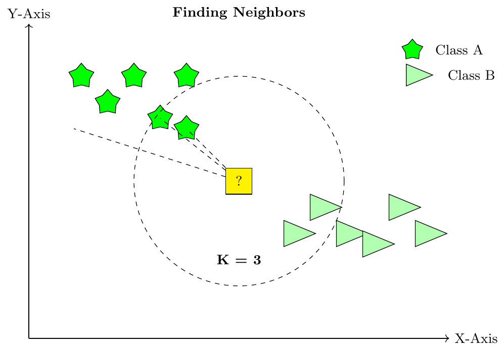
Distance Metrics in k-NN
k-NN classification/regression relies on the notion of distance to identify nearest neighbors. Common distance metrics:
Euclidean Distance (L2 norm): \[ d(\mathbf{x}, \mathbf{y}) = \sqrt{\sum_{i=1}^{n} (x_i - y_i)^2} \] Most common; sensitive to scale and outliers.
Manhattan Distance (L1 norm): \[ d(\mathbf{x}, \mathbf{y}) = \sum_{i=1}^{n} |x_i - y_i| \] Less sensitive to outliers; distances are sum of absolute differences.
Minkowski Distance: Generalized metric: \[ d(\mathbf{x}, \mathbf{y}) = \left(\sum_{i=1}^{n} |x_i - y_i|^p\right)^{1/p} \] Special cases: \(p=1\) → Manhattan, \(p=2\) → Euclidean.
Key Point: Feature scaling is important because large-magnitude features dominate Euclidean distance.
Compute distances between points \(A=(1,2)\) and \(B=(4,6)\):
Euclidean: \(\sqrt{(4-1)^2 + (6-2)^2} = \sqrt{9+16} = \sqrt{25} = 5\)
Manhattan: \(|4-1| + |6-2| = 3 + 4 = 7\)
Minkowski with \(p=3\): \(((3)^3 + (4)^3)^{1/3} = (27+64)^{1/3} = 91^{1/3} \approx 4.48\)
Choice of k and Model Complexity
Small \(k\) (e.g., 1): Model follows data closely, low bias, high variance, sensitive to noise.
Large \(k\): Smoother decision boundaries, higher bias, lower variance, may underfit.
Trade-off: Choose \(k\) using cross-validation to balance bias and variance.
Graphical Intuition:
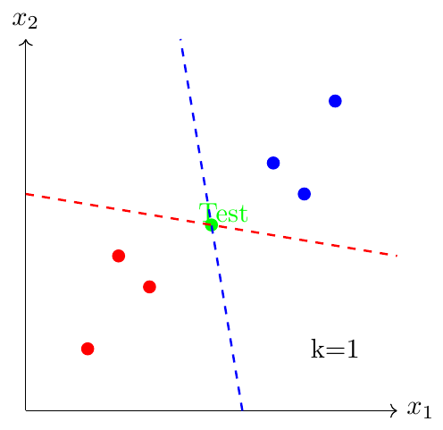
Given 9 points in 2D with two classes (0 and 1). Test point at center:
For \(k=1\): Closest neighbor is class 0 → prediction 0
For \(k=5\): 3 neighbors class 1, 2 neighbors class 0 → prediction 1
Observation: Increasing \(k\) can change prediction and smooth decision boundary.
Effect of Dimensionality on Performance
As the number of features (dimensions) increases:
Distances between points become similar (curse of dimensionality)
Nearest neighbors may be far away → poor generalization
Feature scaling becomes critical.
Dimensionality reduction (PCA, feature selection) improves performance.
Intuition: In high dimensions, most points lie near the corners of a hypercube; Euclidean distance loses discriminative power.
Consider points in 10D: \(x_1=(1,1,...,1), x_2=(2,2,...,2)\). Compute Euclidean distance:
\[ d = \sqrt{\sum_{i=1}^{10} (2-1)^2} = \sqrt{10} \approx 3.16 \]
If all 100 points are randomly distributed in 10D cube $[0,10]^10$, nearest neighbor distances are around 7-8 units. Distances become similar → difficulty in distinguishing neighbors → accuracy drops.
Naive Bayes Classifier
Bayes’ Theorem and Conditional Independence
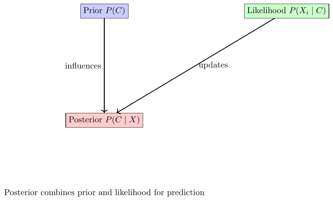
Bayes’ theorem provides a way to update our belief about a class $C$ given observed features $X = (X_1, X_2, \dots, X_n)$:
\[ P(C \mid X) = \frac{P(X \mid C) P(C)}{P(X)} \]
Explanation:
$P(C)$ is the prior probability of class $C$, representing our knowledge before seeing data.
$P(X \mid C)$ is the likelihood: probability of observing $X$ assuming class $C$.
$P(X)$ is the marginal probability of features: ensures probabilities sum to 1.
$P(C \mid X)$ is the posterior: updated probability of class $C$ after observing features.
Naive Bayes assumes features are conditionally independent given the class:
\[ P(X \mid C) = \prod_{i=1}^n P(X_i \mid C) \]
This reduces the exponential complexity of joint probability estimation to linear, making computation feasible.
A weather dataset for predicting PlayTennis has features Outlook and Humidity. Suppose:
$P(\text{Yes}) = 0.6$, $P(\text{No}) = 0.4$
$P(\text{Sunny} \mid \text{Yes}) = 0.3$, $P(\text{High} \mid \text{Yes}) = 0.4$
Then posterior for $C=\text{Yes}$:
\[ P(\text{Yes} \mid X) \propto 0.6 \cdot 0.3 \cdot 0.4 = 0.072 \]
Compute similarly for No and select the class with higher posterior.
Gaussian, Multinomial, and Bernoulli Naive Bayes
For continuous features $X_i \in \mathbb{R}$, model the likelihood as a Gaussian:
\[ P(X_i \mid C) = \frac{1}{\sqrt{2\pi \sigma_{iC}^2}} \exp\Bigg[-\frac{(X_i - \mu_{iC})^2}{2\sigma_{iC}^2}\Bigg] \]
Posterior:
\[ P(C \mid X) \propto P(C) \prod_{i=1}^n P(X_i \mid C) \]
Reasoning: This allows modeling continuous features without discretization.
Used for discrete count data (e.g., word frequencies in documents):
\[ P(X \mid C) = \frac{(\sum_i X_i)!}{\prod_i X_i!} \prod_i \theta_{iC}^{X_i} \]
where $\theta_{iC} = P(\text{word}_i \mid C)$.
For binary features $X_i \in \{0,1\}$:
\[ P(X_i \mid C) = \theta_{iC}^{X_i} (1-\theta_{iC})^{1-X_i} \]
Useful when modeling presence/absence of features.
Email spam classification with binary features: \[ X_1 = \text{“contains ‘offer’”}, X_2 = \text{“contains ‘free’”} \]
Given $P(\text{Spam})=0.4$, $P(X_1=1\mid \text{Spam})=0.7$, $P(X_2=1\mid \text{Spam})=0.6$, test email: $X_1=1, X_2=0$.
\[ P(\text{Spam} \mid X) \propto 0.4 \cdot 0.7 \cdot (1-0.6) = 0.112 \]
Similarly compute $P(\text{Ham} \mid X)$ and choose higher.
Parameter Estimation and MAP Decision Rule
Definition: The MAP decision rule selects the class \(C\) that is most probable given the observed features \(X = (X_1, X_2, \dots, X_n)\). Formally:
\[ \hat{C} = \arg \max_C P(C \mid X) \]
Using Bayes' Theorem:
\[ P(C \mid X) = \frac{P(X \mid C) P(C)}{P(X)} \]
Since \(P(X)\) is the same for all classes, the MAP decision reduces to:
\[ \hat{C} = \arg \max_C P(C) P(X \mid C) \]
Assuming conditional independence of features (Naive Bayes assumption):
\[ P(X \mid C) = \prod_{i=1}^n P(X_i \mid C) \quad \Rightarrow \quad \hat{C} = \arg \max_C P(C) \prod_{i=1}^n P(X_i \mid C) \]
Reasoning:
The MAP rule balances prior knowledge \(P(C)\) with the likelihood of the observed features \(P(X \mid C)\).
It chooses the class that is most likely given the evidence, not just the one with the highest prior probability.
Example: Suppose a dataset has two classes, \(C_1\) and \(C_2\), with priors \(P(C_1)=0.4, P(C_2)=0.6\). For a new observation \(X\), the likelihoods are \(P(X\mid C_1)=0.5\) and \(P(X\mid C_2)=0.3\).
\[ \text{MAP decision: } \hat{C} = \arg \max_C P(C) P(X\mid C) = \arg \max \{0.4 \cdot 0.5, 0.6 \cdot 0.3\} = \arg \max \{0.2, 0.18\} = C_1 \]
Hence, the new observation is classified as \(C_1\) even though \(C_2\) had higher prior probability.
Goal: Estimate the parameters of the Naive Bayes model from data using Maximum Likelihood Estimation (MLE).
1. Multinomial Naive Bayes (word counts): \[ \hat{\theta}_{iC} = P(\text{word}_i \mid C) = \frac{\text{count(word}_i \text{ in class } C)}{\sum_j \text{count(word}_j \text{ in class } C)} \]
$\hat{\theta}_{iC}$ = probability of word \(i\) appearing in class \(C\)
Used in text classification (Bag-of-Words, TF–IDF)
2. Bernoulli Naive Bayes (binary presence/absence): \[ \hat{\theta}_{iC} = P(X_i = 1 \mid C) = \frac{\text{count}(X_i=1 \text{ and } C)}{\text{count}(C)} \]
$\hat{\theta}_{iC}$ = probability that feature \(i\) is present in class \(C\)
Features are Yes/No, Present/Absent, 0/1
3. Gaussian Naive Bayes (continuous features):
\[ \hat{\mu}_{iC} = \frac{1}{n_C} \sum_{j:X_j \in C} X_{ij}, \qquad \hat{\sigma}_{iC}^2 = \frac{1}{n_C} \sum_{j:X_j \in C} (X_{ij}-\hat{\mu}_{iC})^2 \]
$\hat{\mu}_{iC}$ = mean of feature \(i\) in class \(C\)
$\hat{\sigma}_{iC}^2$ = variance of feature \(i\) in class \(C\)
Weather dataset for tennis decision:
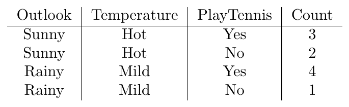
Estimate $P(\text{PlayTennis=Yes} \mid X=\text{Sunny, Hot})$:
\[ P(\text{Yes} \mid X) \propto P(\text{Yes}) P(\text{Sunny}\mid \text{Yes}) P(\text{Hot}\mid \text{Yes}) = \frac{7}{10} \cdot \frac{3}{7} \cdot \frac{3}{7} \approx 0.184 \]
Similarly compute $P(\text{No} \mid X)$ and choose class with higher posterior.
A medical dataset has patients with a symptom \(S\) and a disease \(D\). Suppose:
\[ P(D=\text{Yes}) = 0.1, \quad P(D=\text{No}) = 0.9 \] \[ P(S=\text{Present}\mid D=\text{Yes}) = 0.8, \quad P(S=\text{Present}\mid D=\text{No}) = 0.2 \]
Compute \(P(D=\text{Yes}\mid S=\text{Present})\).
Solution:
\[ P(D=\text{Yes}\mid S) = \frac{P(S\mid D=\text{Yes})P(D=\text{Yes})}{P(S)} \]
First, compute marginal \(P(S)\):
\[ P(S) = P(S\mid D=\text{Yes})P(D=\text{Yes}) + P(S\mid D=\text{No})P(D=\text{No}) = 0.8 \cdot 0.1 + 0.2 \cdot 0.9 = 0.26 \]
\[ \Rightarrow P(D=\text{Yes}\mid S) = \frac{0.8 \cdot 0.1}{0.26} \approx 0.308 \]
Interpretation: Even though the symptom is present, the probability of disease is only 30.8%.
Suppose we have a dataset of students with features: hours studied \(X_1\) and marks obtained \(X_2\), and class \(C = \{\text{Pass}, \text{Fail}\}\).
Data statistics: \[ \text{Pass: } \mu_{X_1}=5, \sigma_{X_1}=1.5, \mu_{X_2}=60, \sigma_{X_2}=10 \] \[ \text{Fail: } \mu_{X_1}=2, \sigma_{X_1}=1, \mu_{X_2}=40, \sigma_{X_2}=5 \]
A student studied 4 hours and scored 55 marks. Using Gaussian NB, compute posterior probabilities (assume \(P(\text{Pass})=0.7, P(\text{Fail})=0.3\)).
Solution:
\[ P(X_1=4 \mid \text{Pass}) = \frac{1}{\sqrt{2\pi (1.5)^2}} e^{-(4-5)^2/(2\cdot1.5^2)} \approx 0.219 \]
\[ P(X_2=55 \mid \text{Pass}) = \frac{1}{\sqrt{2\pi 10^2}} e^{-(55-60)^2/(2\cdot10^2)} \approx 0.038 \]
\[ P(\text{Pass} \mid X_1=4,X_2=55) \propto 0.7 \cdot 0.219 \cdot 0.038 \approx 0.00583 \]
Similarly for Fail:
\[ P(X_1=4 \mid \text{Fail}) \approx 0.054, \quad P(X_2=55 \mid \text{Fail}) \approx 0.00027 \]
\[ P(\text{Fail} \mid X_1,X_2) \propto 0.3 \cdot 0.054 \cdot 0.00027 \approx 0.0000044 \]
Decision: Classify as Pass because posterior is higher.
Suppose we have 2 classes: Spam and Ham, and vocabulary: {“win”, “free”, “offer”}. Training counts:
\[ \text{Spam: } \text{win}=3, \text{free}=4, \text{offer}=2, \text{total words}=9 \] \[ \text{Ham: } \text{win}=1, \text{free}=0, \text{offer}=1, \text{total words}=4 \]
Compute probability that a new message containing “win free” is Spam (assume \(P(\text{Spam})=0.6, P(\text{Ham})=0.4\)).
Solution:
\[ P(\text{win free}\mid \text{Spam}) = \frac{3}{9} \cdot \frac{4}{9} = 0.148 \]
\[ P(\text{win free}\mid \text{Ham}) = \frac{1}{4} \cdot \frac{0}{4} = 0 \]
\[ P(\text{Spam}\mid \text{message}) \propto 0.6 \cdot 0.148 = 0.0888 \]
Decision: Message classified as Spam.
Email classification with 2 features: \(X_1=\) contains “offer”, \(X_2=\) contains “free” (binary). Training statistics:
\[ P(X_1=1\mid \text{Spam})=0.7, P(X_2=1\mid \text{Spam})=0.6 \] \[ P(X_1=1\mid \text{Ham})=0.1, P(X_2=1\mid \text{Ham})=0.05 \] \[ P(\text{Spam})=0.4, P(\text{Ham})=0.6 \]
Test email: \(X_1=1, X_2=0\)
Solution:
\[ P(\text{Spam}\mid X) \propto 0.4 \cdot 0.7 \cdot (1-0.6) = 0.112 \]
\[ P(\text{Ham}\mid X) \propto 0.6 \cdot 0.1 \cdot (1-0.05) = 0.057 \]
Decision: Classify as Spam.
Weather dataset with features: Outlook (Sunny, Rainy) and Temperature (Hot, Mild). Counts:
\[ P(\text{PlayTennis=Yes}) = 0.7, \quad P(\text{PlayTennis=No}) = 0.3 \]
\[ P(\text{Sunny}\mid \text{Yes})=0.5, P(\text{Hot}\mid \text{Yes})=0.6 \]
\[ P(\text{Sunny}\mid \text{No})=0.2, P(\text{Hot}\mid \text{No})=0.5 \]
Test instance: \(X = (\text{Sunny, Hot})\)
Solution:
\[ P(\text{Yes}\mid X) \propto 0.7 \cdot 0.5 \cdot 0.6 = 0.21 \]
\[ P(\text{No}\mid X) \propto 0.3 \cdot 0.2 \cdot 0.5 = 0.03 \]
Decision: Predict PlayTennis = Yes (MAP estimate).
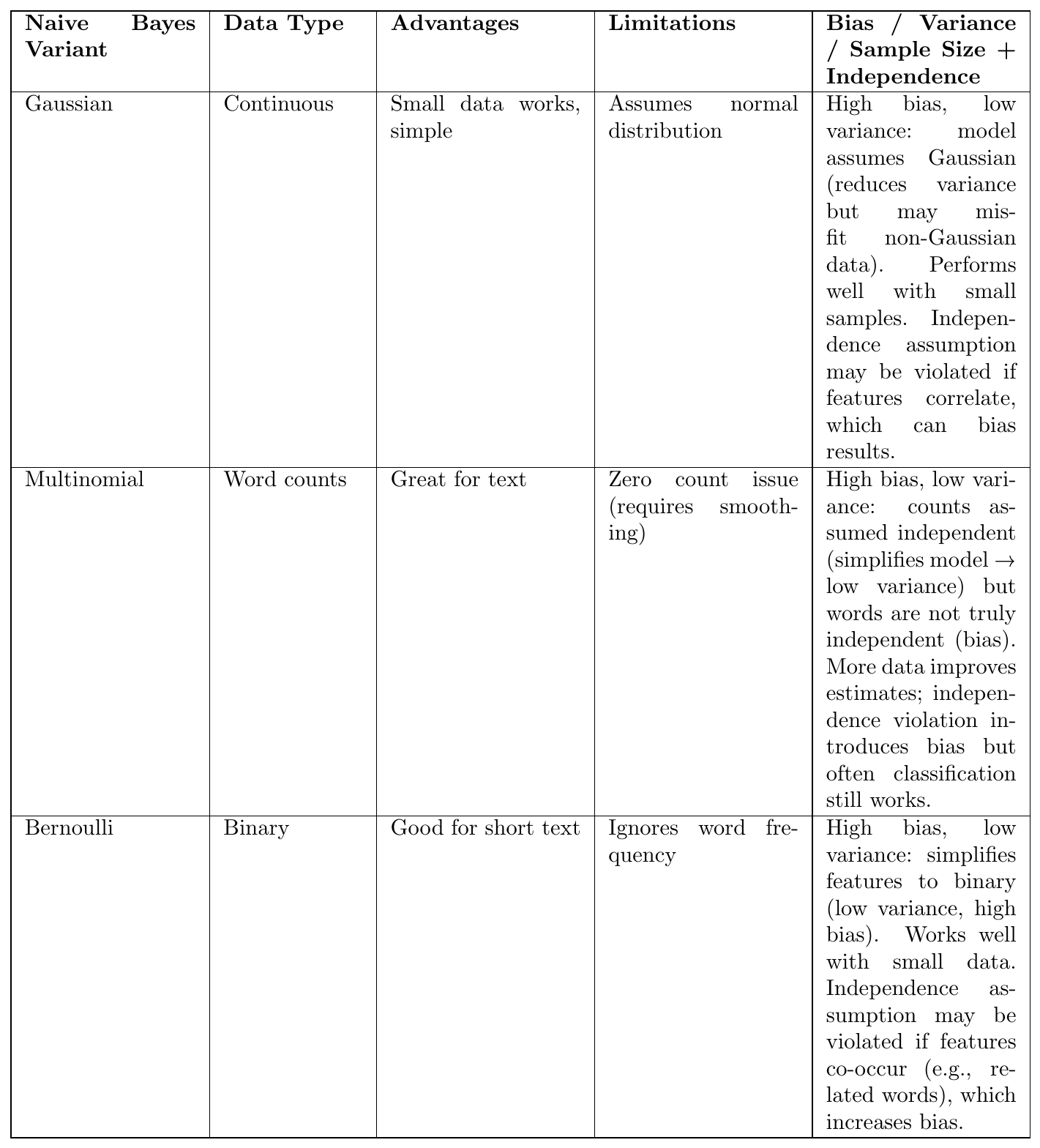
Naive Bayes variants with reasons for bias/variance/sample-size behavior and independence effects.