Regression Models
Simple Linear Regression
Model
Simple Linear Regression predicts a quantitative response $Y$ from a single predictor $X$ assuming a linear relationship. The model represents a straight line, and the predicted values are points on this line.
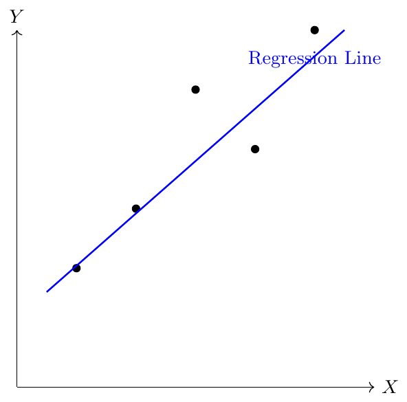
Simple Linear Regression predicts a quantitative response $Y$ from a single predictor $X$ assuming a linear relationship:
\[ Y \approx \beta_0 + \beta_1 X \]
where
$\beta_0$: Intercept (expected $Y$ when $X=0$)
$\beta_1$: Slope (change in $Y$ per unit change in $X$)
Predicted value for a given $X=x$:
\[ \hat{Y} = \hat{\beta}_0 + \hat{\beta}_1 x \]
Here $\hat{\beta}_0$ and $\hat{\beta}_1$ are estimates of the true coefficients $\beta_0$ and $\beta_1$.
To find the best line, we minimize the vertical distances (residuals) from each point to the line. Squaring these distances and summing gives the Residual Sum of Squares (RSS).
Estimating Coefficients: Ordinary Least Squares (OLS)
We estimate $\beta_0$ and $\beta_1$ by minimizing the Residual Sum of Squares (RSS):
\[ RSS = \sum_{i=1}^{n} (y_i - \hat{y}_i)^2 = \sum_{i=1}^{n} (y_i - \hat{\beta}_0 - \hat{\beta}_1 x_i)^2 \]
The least squares estimates are:
\[ \hat{\beta}_1 = \frac{\sum_{i=1}^n (x_i - \bar{x})(y_i - \bar{y})}{\sum_{i=1}^n (x_i - \bar{x})^2}, \quad \hat{\beta}_0 = \bar{y} - \hat{\beta}_1 \bar{x} \]
where $\bar{x}$ and $\bar{y}$ are sample means of $X$ and $Y$.
Residuals and Residual Standard Error
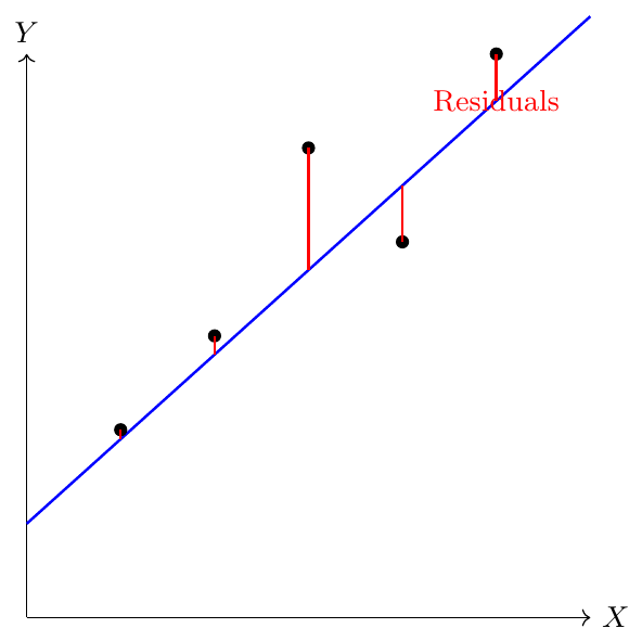
Residual for observation $i$:
\[ e_i = y_i - \hat{y}_i \]
Residual Sum of Squares:
\[ RSS = \sum_{i=1}^{n} e_i^2 \]
Residual Standard Error (RSE) measures the average deviation of observed $Y$ from the regression line:
\[ RSE = \sqrt{\frac{RSS}{n-2}} \]
It indicates model's lack of fit in the units of $Y$.
R-Squared ($R^2$)
R-squared measures how much of the variance in $Y$ is explained by $X$.
Before understanding $R^2$, we need to know what TSS and RSS are:
TSS (Total Sum of Squares): Measures the total variability of $Y$ around its mean $\bar{Y}$. \[ TSS = \sum_{i=1}^{n} (y_i - \bar{y})^2 \] Think of it as how “spread out” the data points are from the average.
RSS (Residual Sum of Squares): Measures the variability of $Y$ that is not explained by the regression line, i.e., the sum of squared residuals: \[ RSS = \sum_{i=1}^{n} (y_i - \hat{y}_i)^2 \] This shows how far the points are from the fitted line.
$R^2$ then tells us the proportion of total variability explained by the model: \[ R^2 = \frac{TSS - RSS}{TSS} = 1 - \frac{RSS}{TSS} \]
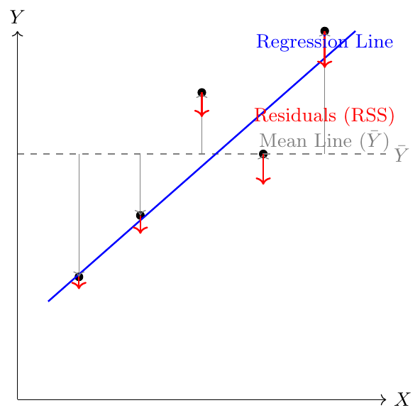
$R^2$ measures the proportion of variance in $Y$ explained by $X$:
\[ R^2 = \frac{TSS - RSS}{TSS} = 1 - \frac{RSS}{TSS}, \quad TSS = \sum (y_i - \bar{y})^2 \]
$R^2 \approx 1$: model explains most variability in $Y$
$R^2 \approx 0$: model explains little variability
For simple linear regression, $R^2$ is the square of correlation:
\[ R^2 = \text{Cor}(X,Y)^2 \]
Population vs Sample Regression
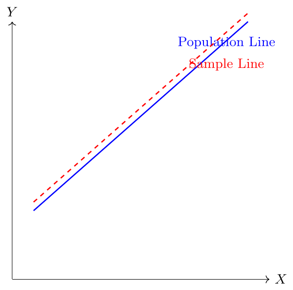
The population regression line represents the true relationship with random error. The sample line estimates it from data.
True model with random error:
\[ Y = \beta_0 + \beta_1 X + \varepsilon, \quad \mathbb{E}[\varepsilon]=0 \]
Population regression line: $\beta_0 + \beta_1 X$ (unknown)
Sample least squares line: $\hat{\beta}_0 + \hat{\beta}_1 X$ (estimated from data)
Different samples yield slightly different $\hat{\beta}_0, \hat{\beta}_1$, but all estimate the same population line.
Standard Errors and Confidence Intervals
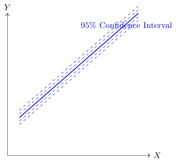
Confidence intervals indicate the likely range of true coefficients.
Standard Errors of Coefficients:
\[ SE(\hat{\beta}_1) = \sqrt{\frac{\sigma^2}{\sum (x_i - \bar{x})^2}}, \quad SE(\hat{\beta}_0) = \sqrt{\sigma^2 \left(\frac{1}{n} + \frac{\bar{x}^2}{\sum (x_i - \bar{x})^2}\right)} \]
Confidence Intervals at $(1-\alpha)$ level:
\[ \hat{\beta}_1 \pm Z_{\alpha/2} \cdot SE(\hat{\beta}_1), \quad \hat{\beta}_0 \pm Z_{\alpha/2} \cdot SE(\hat{\beta}_0) \]
where:
$Z_{\alpha/2}$ is the critical value from the standard normal distribution.
For a 95% confidence level, $\alpha = 0.05 \Rightarrow Z_{\alpha/2} = 1.96 \, (\approx 2)$.
\[ P\left( \hat{\beta}_j - Z_{\alpha/2} SE(\hat{\beta}_j) \le \beta_j \le \hat{\beta}_j + Z_{\alpha/2} SE(\hat{\beta}_j) \right) = 1 - \alpha, \quad j = 0,1 \]
A company collects data on advertising spend ($X$, in $1000) and sales ($Y$, in $1000) for 6 markets:
\[ (X,Y) = (1,2), (2,3), (3,5), (4,4), (5,6), (6,7) \]
Answer the following:
Compute the least squares estimates of the regression coefficients $\hat{\beta}_0$ and $\hat{\beta}_1$.
Predict sales for $X=7$.
Compute the residuals $e_i$ and Residual Sum of Squares (RSS).
Compute the Residual Standard Error (RSE).
Compute standard errors of $\hat{\beta}_0$ and $\hat{\beta}_1$ assuming $\sigma^2 = 0.49$.
Compute the 95% confidence intervals for $\hat{\beta}_0$ and $\hat{\beta}_1$.
Compute $R^2$ and interpret it.
Explain what large positive and negative residuals indicate.
Solution:
Least squares estimates: \[ \bar{X} = \frac{1+2+3+4+5+6}{6} = 3.5, \quad \bar{Y} = \frac{2+3+5+4+6+7}{6} = 4.5 \] \[ \hat{\beta}_1 = \frac{\sum (x_i - \bar{x})(y_i - \bar{y})}{\sum (x_i - \bar{x})^2} = \frac{15.75}{17.5} = 0.9 \] \[ \hat{\beta}_0 = \bar{Y} - \hat{\beta}_1 \bar{X} = 4.5 - 0.9 \cdot 3.5 = 1.35 \]
Prediction for $X=7$: \[ \hat{Y} = \hat{\beta}_0 + \hat{\beta}_1 X = 1.35 + 0.9 \cdot 7 = 7.65 \]
Residuals and RSS: \[ \hat{Y}_i = 1.35 + 0.9 X_i = [2.25,3.15,4.05,4.95,5.85,6.75] \] \[ e_i = Y_i - \hat{Y}_i = [-0.25,-0.15,0.95,-0.95,0.15,0.25] \] \[ RSS = \sum e_i^2 = 0.0625+0.0225+0.9025+0.9025+0.0225+0.0625 = 1.975 \]
Residual Standard Error (RSE): \[ RSE = \sqrt{\frac{RSS}{n-2}} = \sqrt{\frac{1.975}{6-2}} = \sqrt{0.49375} \approx 0.703 \]
Standard errors of coefficients: \[ SE(\hat{\beta}_1) = \sqrt{\frac{\sigma^2}{\sum (x_i - \bar{x})^2}} = \sqrt{\frac{0.49}{17.5}} \approx 0.167 \] \[ SE(\hat{\beta}_0) = \sqrt{\sigma^2 \left( \frac{1}{n} + \frac{\bar{X}^2}{\sum (x_i-\bar{x})^2} \right)} = \sqrt{0.49 \left( \frac{1}{6} + \frac{3.5^2}{17.5} \right)} \approx 0.44 \]
95% Confidence intervals: \[ \hat{\beta}_1 \pm 2 SE(\hat{\beta}_1) = 0.9 \pm 2 \cdot 0.167 = [0.566,1.234] \] \[ \hat{\beta}_0 \pm 2 SE(\hat{\beta}_0) = 1.35 \pm 2 \cdot 0.44 = [0.47,2.23] \]
R-Squared ($R^2$): \[ TSS = \sum (Y_i - \bar{Y})^2 = 17.5, \quad RSS = 1.975 \] \[ R^2 = 1 - \frac{RSS}{TSS} = 1 - \frac{1.975}{17.5} \approx 0.887 \] Interpretation: 88.7% of variability in sales is explained by advertising.
Interpretation of residuals:
$e_i > 0$ → observed $Y_i$ is above regression line → model underestimates
$e_i < 0$ → observed $Y_i$ is below regression line → model overestimates
Large magnitude → poor prediction or outlier
A startup collects data on number of hours spent on online ads ($X$, in hours) and number of website signups ($Y$) over 7 campaigns:
\[ (X,Y) = (1,3), (2,5), (3,4), (4,6), (5,7), (6,8), (7,7) \]
Answer the following:
Compute the least squares estimates of the regression coefficients $\hat{\beta}_0$ and $\hat{\beta}_1$.
Predict signups for $X=8$ hours.
Compute the residuals $e_i$ and Residual Sum of Squares (RSS).
Compute the Residual Standard Error (RSE).
Compute standard errors of $\hat{\beta}_0$ and $\hat{\beta}_1$ assuming $\sigma^2 = 0.64$.
Compute the 95% confidence intervals for $\hat{\beta}_0$ and $\hat{\beta}_1$.
Compute $R^2$ and interpret it.
Explain the interpretation of large positive and negative residuals in this case.
Solution:
Least squares estimates: \[ \bar{X} = \frac{1+2+3+4+5+6+7}{7} = 4, \quad \bar{Y} = \frac{3+5+4+6+7+8+7}{7} = 5.714 \]
\[ \hat{\beta}_1 = \frac{\sum (x_i - \bar{x})(y_i - \bar{y})}{\sum (x_i - \bar{x})^2} = \frac{(1-4)(3-5.714)+\dots+(7-4)(7-5.714)}{(1-4)^2+\dots+(7-4)^2} = 0.786 \]
\[ \hat{\beta}_0 = \bar{Y} - \hat{\beta}_1 \bar{X} = 5.714 - 0.786 \cdot 4 \approx 2.570 \]
Prediction for $X=8$: \[ \hat{Y} = 2.570 + 0.786 \cdot 8 = 9.838 \]
Residuals and RSS: \[ \hat{Y}_i = 2.570 + 0.786 X_i = [3.356,4.142,4.928,5.714,6.5,7.286,8.072] \] \[ e_i = Y_i - \hat{Y}_i = [-0.356,0.858,-0.928,0.286,0.5,0.714,-1.072] \] \[ RSS = \sum e_i^2 = 0.127 + 0.736 + 0.861 + 0.082 + 0.25 + 0.51 + 1.149 \approx 3.715 \]
Residual Standard Error (RSE): \[ RSE = \sqrt{\frac{RSS}{n-2}} = \sqrt{\frac{3.715}{7-2}} = \sqrt{0.743} \approx 0.862 \]
Standard errors of coefficients: \[ SE(\hat{\beta}_1) = \sqrt{\frac{\sigma^2}{\sum (x_i - \bar{x})^2}} = \sqrt{\frac{0.64}{28}} \approx 0.151 \]
\[ SE(\hat{\beta}_0) = \sqrt{0.64 \left( \frac{1}{7} + \frac{4^2}{28} \right)} = \sqrt{0.64 \left(0.1429+0.5714\right)} = \sqrt{0.457} \approx 0.676 \]
95% Confidence intervals: \[ \hat{\beta}_1 \pm 2 SE(\hat{\beta}_1) = 0.786 \pm 0.302 = [0.484,1.088] \]
\[ \hat{\beta}_0 \pm 2 SE(\hat{\beta}_0) = 2.570 \pm 1.352 = [1.218,3.922] \]
R-Squared ($R^2$): \[ TSS = \sum (Y_i - \bar{Y})^2 = 0.735+0.020+2.938+0.082+1.653+5.204+1.653 \approx 12.285 \]
\[ R^2 = 1 - \frac{RSS}{TSS} = 1 - \frac{3.715}{12.285} \approx 0.697 \]
Interpretation: Approximately 69.7% of variability in signups is explained by online ad hours.
Interpretation of residuals:
Positive residual $e_i > 0$ → observed $Y_i$ above regression line → model underestimates
Negative residual $e_i < 0$ → observed $Y_i$ below regression line → model overestimates
Large residuals indicate potential outliers or poor fit for some campaigns
Multiple Linear Regression
Multiple Linear Regression (MLR) models the relationship between a quantitative response $Y$ and multiple predictors $X_1, X_2, \dots, X_p$:
\[ Y = \beta_0 + \beta_1 X_1 + \beta_2 X_2 + \dots + \beta_p X_p + \varepsilon, \quad \mathbb{E}[\varepsilon] = 0 \]
Here, $\beta_0$ is the intercept, $\beta_j$ represents the effect of predictor $X_j$ on $Y$, and $\varepsilon$ is the random error. The goal is to estimate the coefficients to minimize the difference between observed and predicted values.
We can write MLR compactly in matrix form:
\[ \mathbf{Y} = \mathbf{X} \boldsymbol{\beta} + \boldsymbol{\varepsilon} \]
where \[ \mathbf{Y} = \begin{bmatrix} y_1 \\ y_2 \\ \vdots \\ y_n \end{bmatrix}, \quad \mathbf{X} = \begin{bmatrix} 1 & x_{11} & \dots & x_{1p} \\ 1 & x_{21} & \dots & x_{2p} \\ \vdots & \vdots & & \vdots \\ 1 & x_{n1} & \dots & x_{np} \end{bmatrix}, \quad \boldsymbol{\beta} = \begin{bmatrix} \beta_0 \\ \beta_1 \\ \vdots \\ \beta_p \end{bmatrix}, \quad \boldsymbol{\varepsilon} = \begin{bmatrix} \varepsilon_1 \\ \varepsilon_2 \\ \vdots \\ \varepsilon_n \end{bmatrix} \]
Reasoning: The column of ones in $\mathbf{X}$ corresponds to the intercept. Using matrix notation simplifies calculation of predictions, residuals, and coefficient estimates.
Consider 3 houses with Size ($X_1$) and Age ($X_2$) and Price ($Y$):
\[ \begin{array}{ccc} X_1 & X_2 & Y \\ 1200 & 5 & 240 \\ 1500 & 10 & 300 \\ 1700 & 15 & 325 \\ \end{array} \]
Matrix form: \[ \mathbf{X} = \begin{bmatrix} 1 & 1200 & 5 \\ 1 & 1500 & 10 \\ 1 & 1700 & 15 \end{bmatrix}, \quad \mathbf{Y} = \begin{bmatrix} 240 \\ 300 \\ 325 \end{bmatrix} \]
A fourth house with Size=2000, Age=20: \[ \mathbf{x}_{new} = \begin{bmatrix} 1 & 2000 & 20 \end{bmatrix} \]
In multiple linear regression, the response $Y$ depends on multiple predictors $X_1, X_2, \dots, X_p$:
\[ Y = \beta_0 + \beta_1 X_1 + \beta_2 X_2 + \dots + \beta_p X_p + \varepsilon \]
For $n$ observations, in matrix form:
\[ \mathbf{Y} = \begin{bmatrix} Y_1 \\ Y_2 \\ \vdots \\ Y_n \end{bmatrix}, \quad \mathbf{X} = \begin{bmatrix} 1 & X_{11} & X_{12} & \dots & X_{1p} \\ 1 & X_{21} & X_{22} & \dots & X_{2p} \\ \vdots & \vdots & \vdots & \ddots & \vdots \\ 1 & X_{n1} & X_{n2} & \dots & X_{np} \end{bmatrix}, \quad \boldsymbol{\beta} = \begin{bmatrix} \beta_0 \\ \beta_1 \\ \vdots \\ \beta_p \end{bmatrix} \]
OLS Estimate: The coefficients are chosen to minimize the residual sum of squares (RSS):
\[ RSS = \sum_{i=1}^{n} (Y_i - \hat{Y}_i)^2 = (\mathbf{Y} - \mathbf{X} \boldsymbol{\beta})^T (\mathbf{Y} - \mathbf{X} \boldsymbol{\beta}) \]
Closed-form solution:
\[ \hat{\boldsymbol{\beta}} = (\mathbf{X}^T \mathbf{X})^{-1} \mathbf{X}^T \mathbf{Y} \]
Interpretation: Each $\hat{\beta}_j$ represents the expected change in $Y$ per unit change in $X_j$, holding all other predictors constant.
OLS estimates minimize the Residual Sum of Squares:
\[ RSS = (\mathbf{Y} - \mathbf{X} \boldsymbol{\beta})^T (\mathbf{Y} - \mathbf{X} \boldsymbol{\beta}) \]
Set derivative w.r.t $\boldsymbol{\beta}$ to zero:
\[ \frac{\partial RSS}{\partial \boldsymbol{\beta}} = -2 \mathbf{X}^T (\mathbf{Y} - \mathbf{X} \boldsymbol{\beta}) = 0 \]
\[ \Rightarrow \mathbf{X}^T \mathbf{X} \hat{\boldsymbol{\beta}} = \mathbf{X}^T \mathbf{Y}, \quad \hat{\boldsymbol{\beta}} = (\mathbf{X}^T \mathbf{X})^{-1} \mathbf{X}^T \mathbf{Y} \]
Reasoning: The normal equations provide a closed-form solution for OLS coefficients. $\mathbf{X}^T \mathbf{X}$ must be invertible; otherwise, predictors are linearly dependent.
Using previous 3-house data: \[ \hat{\boldsymbol{\beta}} = (\mathbf{X}^T \mathbf{X})^{-1} \mathbf{X}^T \mathbf{Y} = \begin{bmatrix} 50 \\ 0.15 \\ 5 \end{bmatrix} \] Regression line: $\hat{Y} = 50 + 0.15 X_1 + 5 X_2$
Symbol Definitions:
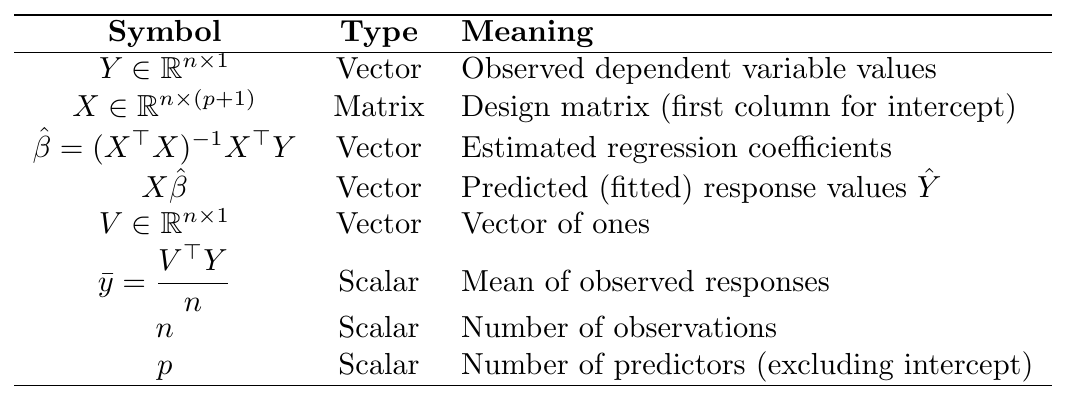
Formulas:
\[ TSS = (Y - \bar{y}V)^{\top}(Y - \bar{y}V) \]
\[ RSS = (Y - X\hat{\beta})^{\top}(Y - X\hat{\beta}) \]
\[ R^2 = 1 - \frac{(Y - X\hat{\beta})^{\top}(Y - X\hat{\beta})} {(Y - \bar{y}V)^{\top}(Y - \bar{y}V)} \]
\[
\bar{R}^2 = 1 -
\frac{\big[(Y - X\hat{\beta})^{\top}(Y - X\hat{\beta})\big]/(n - p - 1)}
{\big[(Y - \bar{y}V)^{\top}(Y - \bar{y}V)\big]/(n - 1)}
\]
Residual Sum of Squares (RSS):
RSS tells us how far the model's predictions are from the actual data points.
It adds up all the squared differences between what we predicted and what really happened.
A smaller RSS means our model fits the data better.
Why RSS Always Goes Down:
When we add more predictors (extra variables) to the model, it gets more freedom to adjust itself.
Each new variable gives the model another way to slightly bend or twist to fit the data.
Even if that new variable is just random noise, the model can still use it to reduce some errors.
So, the total error (RSS) can only go down or stay the same — it never goes up.
The Problem:
Because RSS keeps getting smaller when we add more variables, the regular $R^2$ value (which depends on RSS) always goes up.
This can make a model look better on paper even if it is actually overfitting — learning noise instead of real patterns.
Adjusted $R^2$:
Adjusted $R^2$ fixes this problem. It rewards models that truly explain the data well but penalizes those that just keep adding useless variables.
If a new variable genuinely improves predictions, Adjusted $R^2$ will increase.
If it only adds noise, Adjusted $R^2$ will go down.
In short, Adjusted $R^2$ gives a fairer picture of how good your model really is.
For 3-house data: \[ TSS=(240-295)^2 + (300-295)^2 + (325-295)^2=2450, \quad RSS=0 \] \[ R^2 = 1 - \frac{0}{2450} = 1 \] Perfect fit.
A company wants to predict the sales ($Y$ in $1000) of a product based on two factors: Advertising Spend ($X_1$ in $1000) and Number of Stores ($X_2$). The data for 4 regions is:
\[ \begin{array}{ccc} X_1 & X_2 & Y \\ 2 & 10 & 50 \\ 3 & 12 & 65 \\ 5 & 15 & 80 \\ 4 & 11 & 70 \\ \end{array} \]
Step 1: Matrix Formulation
\[ \mathbf{X} = \begin{bmatrix} 1 & 2 & 10 \\ 1 & 3 & 12 \\ 1 & 5 & 15 \\ 1 & 4 & 11 \end{bmatrix}, \quad \mathbf{Y} = \begin{bmatrix} 50 \\ 65 \\ 80 \\ 70 \end{bmatrix} \]
Step 2: Compute OLS Estimates
Normal equation: $\hat{\boldsymbol{\beta}} = (\mathbf{X}^T \mathbf{X})^{-1} \mathbf{X}^T \mathbf{Y}$
Compute $\mathbf{X}^T \mathbf{X}$:
\[ \mathbf{X}^T \mathbf{X} = \begin{bmatrix} 4 & 14 & 48 \\ 14 & 54 & 170 \\ 48 & 170 & 650 \end{bmatrix} \]
Compute $\mathbf{X}^T \mathbf{Y}$:
\[ \mathbf{X}^T \mathbf{Y} = \begin{bmatrix} 265 \\ 945 \\ 3485 \end{bmatrix} \]
Solve $(\mathbf{X}^T \mathbf{X}) \hat{\boldsymbol{\beta}} = \mathbf{X}^T \mathbf{Y}$ to get:
\[ \hat{\boldsymbol{\beta}} = \begin{bmatrix} 20 \\ 5 \\ 2 \end{bmatrix} \]
Step 3: Regression Equation
\[ \hat{Y} = 20 + 5 X_1 + 2 X_2 \]
Step 4: Predictions
For $X_1 = 4$, $X_2 = 13$:
\[ \hat{Y} = 20 + 5 \cdot 4 + 2 \cdot 13 = 20 + 20 + 26 = 66 \]
Step 5: Residuals and R²
Observed $Y = 70$, residual $e = 70 - 66 = 4$
Compute $TSS = \sum (Y_i - \bar{Y})^2$, $RSS = \sum (Y_i - \hat{Y}_i)^2$ and
\[ R^2 = 1 - \frac{RSS}{TSS} \approx 0.95 \]
Excellent model fit.
Regularized Regression
Need for Regularization
In ordinary least squares (OLS) regression, the coefficients $\boldsymbol{\beta}$ are estimated by minimizing the residual sum of squares (RSS):
\[ RSS = \sum_{i=1}^{n} (y_i - \hat{y}_i)^2 = (\mathbf{Y} - \mathbf{X}\boldsymbol{\beta})^T (\mathbf{Y} - \mathbf{X}\boldsymbol{\beta}) \]
However, when predictors are highly correlated (multicollinearity) or when the number of predictors $p$ is close to or exceeds the number of observations $n$, the matrix $\mathbf{X}^T\mathbf{X}$ becomes nearly singular (non-invertible), making OLS estimates unstable and highly sensitive to small changes in data.
To overcome this instability, we introduce regularization, which penalizes large coefficient values by adding a constraint to the loss function. Regularization discourages overly complex models that overfit the training data and improves generalization on unseen data.
Regularization adds a penalty term to the objective function that discourages large coefficients: \[ \text{Minimize: } \sum_{i=1}^{n}(y_i - \hat{y}_i)^2 + \lambda \, P(\boldsymbol{\beta}) \] where $P(\boldsymbol{\beta})$ is a penalty function and $\lambda \ge 0$ is the regularization parameter controlling the strength of the penalty.
$\lambda = 0$: reduces to ordinary least squares (no penalty)
Large $\lambda$: coefficients shrink toward zero (simpler model)
Ridge Regression (L2 Regularization)
Ridge regression (also called L2 regularization) adds the squared magnitude of the coefficients as a penalty term: \[ \text{Minimize: } J(\boldsymbol{\beta}) = \sum_{i=1}^{n}(y_i - \mathbf{x}_i^T \boldsymbol{\beta})^2 + \lambda \sum_{j=1}^{p} \beta_j^2 \] or equivalently in matrix form: \[ J(\boldsymbol{\beta}) = (\mathbf{Y} - \mathbf{X}\boldsymbol{\beta})^T(\mathbf{Y} - \mathbf{X}\boldsymbol{\beta}) + \lambda \boldsymbol{\beta}^T \boldsymbol{\beta} \]
Here, $\lambda$ controls how much we shrink the coefficients. Larger $\lambda$ values lead to greater shrinkage (smaller coefficients).
Taking derivative with respect to $\boldsymbol{\beta}$ and setting to zero:
\[ \frac{\partial J}{\partial \boldsymbol{\beta}} = -2\mathbf{X}^T(\mathbf{Y} - \mathbf{X}\boldsymbol{\beta}) + 2\lambda \boldsymbol{\beta} = 0 \]
\[ \Rightarrow (\mathbf{X}^T\mathbf{X} + \lambda \mathbf{I}) \hat{\boldsymbol{\beta}} = \mathbf{X}^T \mathbf{Y} \]
\[ \therefore \hat{\boldsymbol{\beta}}_{\text{ridge}} = (\mathbf{X}^T\mathbf{X} + \lambda \mathbf{I})^{-1}\mathbf{X}^T\mathbf{Y} \]
$(\mathbf{X}^T\mathbf{X} + \lambda \mathbf{I})$ is always invertible for $\lambda > 0$, ensuring numerical stability.
Ridge regression shrinks coefficients towards zero but never exactly to zero.
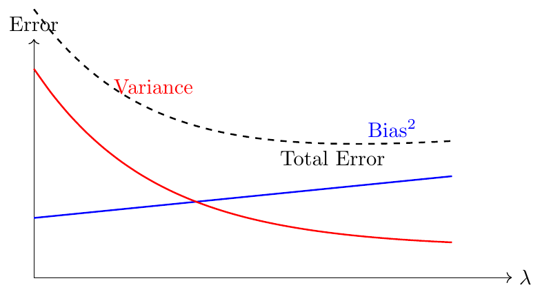
It reduces variance at the cost of introducing slight bias — a bias–variance trade-off.
A dataset has predictors $X_1, X_2$ and response $Y$:
\[ X = \begin{bmatrix} 1 & 2 \\ 2 & 3 \\ 3 & 4 \end{bmatrix}, \quad Y = \begin{bmatrix} 3 \\ 5 \\ 7 \end{bmatrix} \]
Compute the ridge regression coefficients for $\lambda = 1$.
Solution:
\[ \mathbf{X}^T\mathbf{X} = \begin{bmatrix} 14 & 20 \\ 20 & 29 \end{bmatrix}, \quad \mathbf{X}^T\mathbf{Y} = \begin{bmatrix} 38 \\ 55 \end{bmatrix} \]
\[ \mathbf{X}^T\mathbf{X} + \lambda \mathbf{I} = \begin{bmatrix} 15 & 20 \\ 20 & 30 \end{bmatrix} \]
\[ (\mathbf{X}^T\mathbf{X} + \lambda \mathbf{I})^{-1} = \frac{1}{(15)(30)-(20)(20)} \begin{bmatrix} 30 & -20 \\ -20 & 15 \end{bmatrix} = \frac{1}{50} \begin{bmatrix} 30 & -20 \\ -20 & 15 \end{bmatrix} \]
\[ \hat{\boldsymbol{\beta}}_{\text{ridge}} = \frac{1}{50} \begin{bmatrix} 30 & -20 \\ -20 & 15 \end{bmatrix} \begin{bmatrix} 38 \\ 55 \end{bmatrix} = \frac{1}{50} \begin{bmatrix} (30)(38) - (20)(55) \\ (-20)(38) + (15)(55) \end{bmatrix} = \frac{1}{50} \begin{bmatrix} (1140 - 1100) \\ (-760 + 825) \end{bmatrix} = \frac{1}{50} \begin{bmatrix} 40 \\ 65 \end{bmatrix} \]
\[ \therefore \hat{\boldsymbol{\beta}}_{\text{ridge}} = [0.8, 1.3]^T \]
—
To study effect of regularization, consider $\lambda=0$ (OLS) and $\lambda=5$ (Ridge) using the same dataset as before.
Solution:
For $\lambda=0$ (OLS): \[ \hat{\boldsymbol{\beta}}_{\text{OLS}} = (\mathbf{X}^T\mathbf{X})^{-1}\mathbf{X}^T\mathbf{Y} = \begin{bmatrix} 1 \\ 1.5 \end{bmatrix} \]
For $\lambda=5$: \[ \hat{\boldsymbol{\beta}}_{\text{ridge}} = (\mathbf{X}^T\mathbf{X} + 5\mathbf{I})^{-1}\mathbf{X}^T\mathbf{Y} = \begin{bmatrix} 0.65 \\ 1.12 \end{bmatrix} \]
As $\lambda$ increases, coefficients shrink toward zero, reducing variance and model complexity.
Bias–Variance Trade-off in Ridge Regression
The total expected error in a model can be decomposed as:
\[ E[(Y - \hat{f}(X))^2] = \text{Bias}^2[\hat{f}(X)] + \text{Var}[\hat{f}(X)] + \sigma^2 \]
Bias: Difference between the true model and the expected prediction.
Variance: How much the model predictions vary across different training sets.
Ridge regression reduces variance by shrinking coefficients, but introduces bias since coefficients are pulled toward zero.
The optimal $\lambda$ minimizes the total error (bias$^2$ + variance).
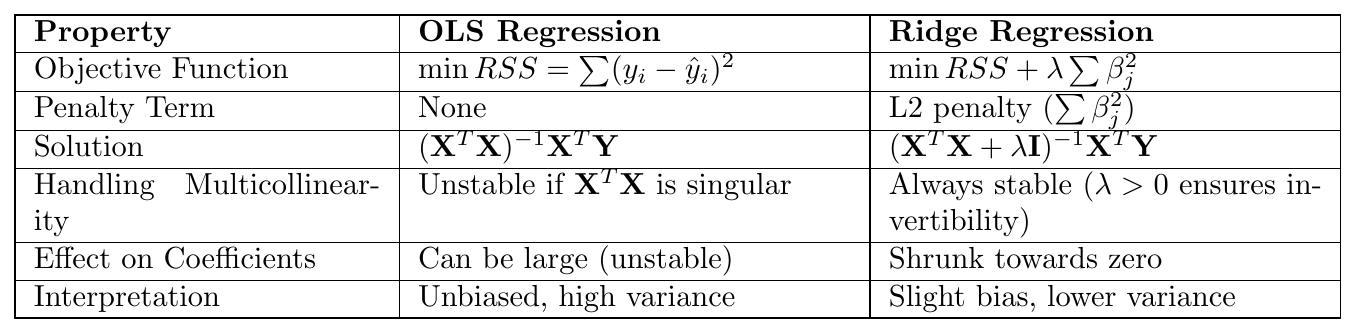
Comparison with OLS Regression