Classification Models - II
Linear Discrimination Analysis (LDA)
Linear Discriminant Analysis (LDA) is a supervised dimensionality reduction technique used in machine learning, statistics, and pattern recognition. It seeks to find a linear projection (a direction or axis) that maximizes the separation between multiple classes while minimizing the spread within each class.
LDA is primarily used for:
Feature reduction: projecting high-dimensional data onto a lower-dimensional subspace.
Classification: improving class separability before applying classifiers such as Logistic Regression or SVM.
Generative Perspective (Bayesian LDA):
This approach treats LDA as a generative model, meaning it attempts to learn how each class generates the data. It models the probability distribution of the features for each class, $p(x|C_k)$, and combines it with the prior probability $P(C_k)$ to compute the posterior probability $P(C_k|x)$ using Bayes’ theorem. In simple terms, the model first learns the underlying data distribution of each class and then predicts which class is most likely to have produced a new observation.Discriminative Perspective (Fisher’s LDA):
This approach treats LDA as a discriminative model, meaning it focuses on finding a boundary that best separates the classes rather than modeling how the data was generated. Fisher’s method seeks a projection direction in which the classes are most distinct — that is, the distance between class means is large while the variation within each class is small. It does not model class probabilities explicitly but directly aims to achieve maximum class separability.
Summary:
In essence, the generative form (Bayesian LDA) focuses on how data is produced by each class,
while the discriminative form (Fisher’s LDA) focuses on how to best separate the classes.
Fisher’s Linear Discriminant Analysis (LDA)
LDA aims to find a direction \( \mathbf{w} \) such that, when data points \( \mathbf{x} \) are projected onto it, the between-class variance is maximized, and the within-class variance is minimized.
The following figures illustrate how LDA transforms data by projecting it onto a line that best separates the classes.
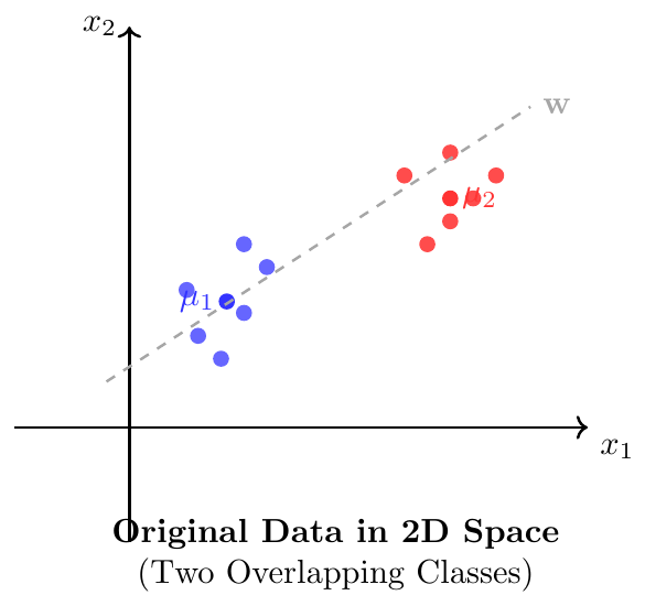
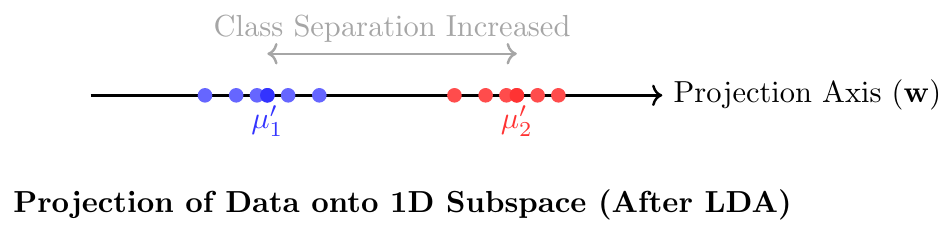
{LDA finds a projection direction $\mathbf{w}$ that maximizes class separability. In the top figure, data from two classes overlap in the 2D space. After projection (bottom figure), the classes are well separated in 1D.}
Fisher’s Linear Discriminant Analysis (LDA) finds a projection direction (or matrix) that maximizes the separation between classes in a lower-dimensional space.
Goal: Find a projection vector $w$ that projects high-dimensional data $X = (X_1, X_2, \ldots, X_p)^T$ onto a one-dimensional line $y = w^T X$ such that samples from different classes are well-separated while samples within the same class remain close.
Intuition:
LDA is not just a classifier — it’s a dimensionality reduction technique that preserves class separability.
For two classes, it finds a single direction $w$ maximizing the ratio of between-class variance to within-class variance.
For $K$ classes, it finds $(K-1)$ optimal directions (columns of $W$).
Two-Class Fisher LDA: Step-by-Step Derivation
Let two classes $C_1$ and $C_2$ have: \[ \mu_1 = \frac{1}{N_1}\sum_{i\in C_1} x^{(i)}, \quad \mu_2 = \frac{1}{N_2}\sum_{i\in C_2} x^{(i)} \] The global mean: \[ \mu = \frac{N_1\mu_1 + N_2\mu_2}{N_1 + N_2} \]
Within-class scatter: \[ S_W = S_1 + S_2, \quad S_k = \sum_{i\in C_k} (x^{(i)} - \mu_k)(x^{(i)} - \mu_k)^T \] represents how samples of the same class are scattered around their mean.
Between-class scatter: \[ S_B = (\mu_1 - \mu_2)(\mu_1 - \mu_2)^T \] represents how far apart the class means are.
We project each sample $x$ onto a line: \[ y = w^T x \]
The projected means: \[ m_1 = w^T \mu_1, \quad m_2 = w^T \mu_2 \]
The projected within-class variance: \[ s_w^2 = w^T S_W w \]
Fisher’s criterion: \[ J(w) = \frac{(m_1 - m_2)^2}{s_w^2} = \frac{w^T S_B w}{w^T S_W w} \]
Goal: Maximize $J(w)$ to find the best discriminant direction.
Maximizing $J(w)$: \[ \max_w \frac{w^T S_B w}{w^T S_W w} \]
This leads to: \[ S_B w = \lambda S_W w \]
Substitute $S_B = (\mu_1 - \mu_2)(\mu_1 - \mu_2)^T$: \[ (\mu_1 - \mu_2)(\mu_1 - \mu_2)^T w = \lambda S_W w \]
This gives the solution: \[ w \propto S_W^{-1}(\mu_1 - \mu_2) \]
Interpretation:
$S_W^{-1}$ “whitens” the data (removes within-class correlation).
$(\mu_1 - \mu_2)$ gives the direction connecting class means.
Hence $w$ points in the direction of maximal class separability.
Numerical Example
Given: \[ \mu_1 = \begin{bmatrix}1\\2\end{bmatrix}, \quad \mu_2 = \begin{bmatrix}3\\4\end{bmatrix}, \quad S_W = \begin{bmatrix}2 & 1\\1 & 2\end{bmatrix} \]
Compute: \[ w = S_W^{-1}(\mu_1 - \mu_2) \] \[ S_W^{-1} = \frac{1}{3} \begin{bmatrix}2 & -1\\-1 & 2\end{bmatrix} \Rightarrow w = \frac{1}{3}\begin{bmatrix}-2\\-2\end{bmatrix} \propto \begin{bmatrix}-1\\-1\end{bmatrix} \]
Decision rule: Project $x$ and classify based on threshold: \[ y = w^T x, \quad \text{assign to } C_1 \text{ if } y < t, \text{ else } C_2 \] where \[ t = \frac{1}{2} w^T (\mu_1 + \mu_2) \]
Multiclass Fisher LDA Derivation
For $K$ classes, we define: \[ S_W = \sum_{k=1}^{K}\sum_{i\in C_k}(x^{(i)} - \mu_k)(x^{(i)} - \mu_k)^T, \quad S_B = \sum_{k=1}^{K} N_k(\mu_k - \mu)(\mu_k - \mu)^T \]
Objective: \[ J(W) = \frac{|W^T S_B W|}{|W^T S_W W|} \]
Optimization leads to the generalized eigenvalue problem: \[ S_B w_i = \lambda_i S_W w_i, \quad i = 1,2,\ldots,K-1 \]
The top $(K-1)$ eigenvectors form the projection matrix: \[ W = [w_1, w_2, \ldots, w_{K-1}] \]
Interpretation:
Each column of $W$ defines one discriminant axis.
The data is projected onto the $(K-1)$-dimensional subspace for maximum separability.
Assumptions of Fisher LDA
Each class is normally distributed (Gaussian).
All classes share the same covariance matrix $\Sigma$.
Classes are linearly separable in some projection space.
$S_W$ is nonsingular or regularized.
Bayesian View of Linear Discriminant Analysis
Assumption: For each class \(C_k\) the class-conditional density is Gaussian with common covariance \(\Sigma\) and mean \(\mu_k\): \[ p(x\mid C_k) = \frac{1}{(2\pi)^{p/2}|\Sigma|^{1/2}} \exp\!\Big( -\tfrac{1}{2}(x-\mu_k)^\top\Sigma^{-1}(x-\mu_k)\Big). \]
Step 1: write the log-likelihood (log of class-conditional density). \[ \log p(x\mid C_k) = -\frac{p}{2}\log(2\pi) -\frac{1}{2}\log|\Sigma| \;-\;\frac{1}{2}(x-\mu_k)^\top\Sigma^{-1}(x-\mu_k). \] The first two terms are constants w.r.t. \(x\) and \(k\) (if \(\Sigma\) is common).
Step 2: expand the quadratic form. Use \[ (x-\mu_k)^\top\Sigma^{-1}(x-\mu_k) = x^\top\Sigma^{-1}x \;-\; 2x^\top\Sigma^{-1}\mu_k \;+\; \mu_k^\top\Sigma^{-1}\mu_k. \] Substitute into the log-likelihood: \[ \log p(x\mid C_k) = -\frac{p}{2}\log(2\pi) -\frac{1}{2}\log|\Sigma| \;-\;\frac{1}{2}x^\top\Sigma^{-1}x \;+\; x^\top\Sigma^{-1}\mu_k \;-\;\frac{1}{2}\mu_k^\top\Sigma^{-1}\mu_k. \]
Step 3: form the log-posterior (discriminant) by adding the log prior. Let the class prior be \(P(C_k)=\pi_k\). Define \[ \delta_k(x) \;=\; \log p(x\mid C_k) + \log\pi_k. \] Hence \[ \delta_k(x) = -\frac{p}{2}\log(2\pi) -\frac{1}{2}\log|\Sigma| -\frac{1}{2}x^\top\Sigma^{-1}x + x^\top\Sigma^{-1}\mu_k -\frac{1}{2}\mu_k^\top\Sigma^{-1}\mu_k + \log\pi_k. \]
Step 4: drop terms that are common to all classes. The terms \(-\tfrac{p}{2}\log(2\pi)\), \(-\tfrac{1}{2}\log|\Sigma|\) and \(-\tfrac{1}{2}x^\top\Sigma^{-1}x\) do not depend on \(k\), so they cancel when comparing \(\delta_i(x)\) vs \(\delta_j(x)\). Removing those common terms (or equivalently adding a constant) yields the simplified discriminant: \[ \boxed{\; \delta_k(x) \;=\; x^\top\Sigma^{-1}\mu_k \;-\; \tfrac{1}{2}\mu_k^\top\Sigma^{-1}\mu_k \;+\; \log\pi_k \;} \] This is an affine (linear + constant) function of \(x\).
Step 5: write the pairwise decision boundary. To find the boundary between class \(C_i\) and \(C_j\) set \(\delta_i(x)=\delta_j(x)\). Rearranging: \[ x^\top\Sigma^{-1}(\mu_i-\mu_j) \;=\; \tfrac{1}{2}\big(\mu_i^\top\Sigma^{-1}\mu_i - \mu_j^\top\Sigma^{-1}\mu_j\big) \;-\; \log\frac{\pi_i}{\pi_j}. \] This is a linear equation in \(x\) (a hyperplane), so the decision boundary is linear.
Remark: If covariances are not equal (\(\Sigma_k\) differ across classes), the quadratic term \(-\tfrac12 x^\top\Sigma_k^{-1}x\) will not cancel across classes and the resulting boundary is generally quadratic — this gives Quadratic Discriminant Analysis (QDA) instead of LDA.
Decision rule: Assign \(x\) to the class \(C_k\) with the largest \(\delta_k(x)\).
Assumptions in Bayesian LDA
$p(x|C_k)$ is Gaussian for all $k$.
All classes share identical covariance $\Sigma$.
Priors $\pi_k$ are known or estimated from sample proportions.
The decision boundaries are linear in $x$.
Example: Bayesian LDA (Two Classes)
Let: \[ \mu_1 = (1,2), \quad \mu_2 = (3,4), \quad \Sigma = I, \quad \pi_1 = \pi_2 = 0.5 \] Then: \[ \delta_k(x) = x^T \mu_k - \frac{1}{2}\mu_k^T \mu_k + \log \pi_k \]
Boundary: \[ x^T(\mu_1 - \mu_2) = \frac{1}{2}(\mu_1^T \mu_1 - \mu_2^T \mu_2) \] Substitute: \[ x^T[-2, -2] = \frac{1}{2}(5 - 25) \Rightarrow x_1 + x_2 = 5 \] Hence, samples with $x_1 + x_2 > 5$ belong to $C_2$; otherwise $C_1$.