The Random Variables
Introduction
Definition: A random variable (RV) is a function that assigns a real number to each outcome in the sample space of a random experiment.
There are two types:
Discrete Random Variable: Takes a countable number of values.
Continuous Random Variable: Takes values in a continuous range.
Examples:
Coin Tossing:
Experiment: Toss a fair coin 3 times.
Sample space: $\{HHH, HHT, HTH, HTT, THH, THT, TTH, TTT\}$
Define $X$ = number of heads. Then $X$ is a discrete RV taking values $\{0,1,2,3\}$.
Dice Roll:
Experiment: Roll a fair 6-sided die once.
Sample space: $\{1,2,3,4,5,6\}$
Define $Y$ = value shown on the die. $Y$ is a discrete RV taking values from 1 to 6.
Card Draw:
Experiment: Draw one card from a deck.
Define $Z = 1$ if red card drawn, $Z = 0$ otherwise.
$Z$ is a discrete RV with values $\{0,1\}$.
Measuring Height:
Experiment: Measure the height of a randomly selected student.
Define $H$ = height in cm. $H$ can take any real value in an interval, e.g., $[120, 200]$.
$H$ is a continuous RV.
Summary: A random variable converts qualitative outcomes into quantitative values for probabilistic analysis.
Overview of Discrete Probability Distributions
A Discrete Random Variable (DRV) is a variable that can take on a countable number of values, each with a corresponding probability.
A Discrete Probability Distribution describes the probability that a discrete random variable takes each of its possible values.
Probability Mass Function (PMF): Let $X$ be a discrete random variable. The function $f(x)$ defined as:
\[ f(x) = P(X = x) \]
is called the Probability Mass Function (PMF), which satisfies:
$f(x) \geq 0$ for all $x$
$\sum_x f(x) = 1$
$P(X = x) = f(x)$
Cumulative Distribution Function (CDF): The cumulative distribution function $F(x)$ gives the probability that $X$ is less than or equal to $x$:
\[ F(x) = P(X \leq x) = \sum_{t \leq x} f(t) \]
Let $X$ be the number of heads observed when a fair coin is tossed 3 times.
Sample Space: Each toss has 2 outcomes: H or T. Total outcomes: $2^3 = 8$ Enumerating outcomes:
0 heads: TTT
1 head: HTT, THT, TTH
2 heads: HHT, HTH, THH
3 heads: HHH
PMF Table: \[ \begin{array}{|c|c|} x & P(X = x) \\ 0 & \frac{1}{8} \\ 1 & \frac{3}{8} \\ 2 & \frac{3}{8} \\ 3 & \frac{1}{8} \\ \end{array} \]
CDF Table: \[ \begin{array}{|c|c|} x & F(x) = P(X \leq x) \\ 0 & \frac{1}{8} \\ 1 & \frac{4}{8} \\ 2 & \frac{7}{8} \\ 3 & 1 \\ \end{array} \]
Let $M$ be the number of employees getting back their own helmets when 3 helmets are randomly returned.
Possible values: $M = 0, 1, 3$
PMF: \[ \begin{array}{|c|c|} m & P(M = m) \\ 0 & \frac{1}{3} \\ 1 & \frac{1}{2} \\ 3 & \frac{1}{6} \\ \end{array} \]
Check: $\frac{1}{3} + \frac{1}{2} + \frac{1}{6} = 1$
This is a valid discrete probability distribution.
A small company buys 2 laptops at random from a shipment of 20, where 3 are defective. Let $X$ be the number of defectives selected.
Total ways to choose 2 laptops out of 20: ${20 \choose 2} = 190$
Now, calculate:
$P(X = 0)$ = Both are non-defective: ${17 \choose 2}/190 = 136/190$
$P(X = 1)$ = One defective, one good: ${3 \choose 1}{17 \choose 1}/190 = 51/190$
$P(X = 2)$ = Both defective: ${3 \choose 2}/190 = 3/190$
PMF Table: \[ \begin{array}{|c|c|} x & P(X = x) \\ 0 & \frac{136}{190} \\ 1 & \frac{51}{190} \\ 2 & \frac{3}{190} \\ \end{array} \]
Check: $\frac{136 + 51 + 3}{190} = 1$
Problem: A car dealership sells a particular foreign car, 50% of which are equipped with side airbags. Let $X$ denote the number of cars with side airbags among the next 4 cars sold.
Determine a formula for the probability distribution of $X$.
Find the cumulative distribution function (CDF) of $X$.
Solution:
We are dealing with a Binomial distribution problem where:
Number of trials: $n = 4$
Probability of success (a car with airbags): $p = 0.5$
Random variable $X$: number of cars with airbags among the next 4 sold
1. Probability Mass Function (PMF)
For a binomial random variable, the PMF is given by:
\[
P(X = x) = \binom{n}{x} p^x (1-p)^{n-x}, \quad x = 0, 1, 2, 3, 4
\]
Substituting $n = 4$ and $p = 0.5$:
\[
P(X = x) = \binom{4}{x} (0.5)^x (0.5)^{4-x} = \binom{4}{x} \cdot (0.5)^4 = \binom{4}{x} \cdot \frac{1}{16}
\]
2. PMF Values: \begin{align*} P(X = 0) &= \frac{1}{16}, & P(X = 1) &= \frac{4}{16}, \\ P(X = 2) &= \frac{6}{16}, & P(X = 3) &= \frac{4}{16}, \\ P(X = 4) &= \frac{1}{16} \end{align*}
3. Probability Distribution Table: \[ \begin{array}{|c|c|} x & P(X = x) \\ 0 & \frac{1}{16} \\ 1 & \frac{4}{16} \\ 2 & \frac{6}{16} \\ 3 & \frac{4}{16} \\ 4 & \frac{1}{16} \\ \end{array} \]
4. Cumulative Distribution Function (CDF): \[ \begin{array}{|c|c|} x & F(x) = P(X \le x) \\ 0 & \frac{1}{16} \\ 1 & \frac{1+4}{16} = \frac{5}{16} \\ 2 & \frac{5+6}{16} = \frac{11}{16} \\ 3 & \frac{11+4}{16} = \frac{15}{16} \\ 4 & \frac{15+1}{16} = 1 \\ \end{array} \]
Overview of Continuous Probability Distributions
A continuous random variable can assume an infinite number of values in a given range. The probability that a continuous random variable takes on any exact value is zero. This is because between any two real numbers, no matter how close, there are infinitely many values.
Example: Consider the heights of people over 21 years of age. The probability that a randomly chosen person is exactly 164 cm tall is 0. However, the probability that the height lies within an interval, say between 163 and 165 cm, is greater than 0.
For a continuous random variable $X$, the probability is computed over an interval: \[ P(a < X < b) = \int_a^b f(x) \, dx \]
Here, $f(x)$ is called the probability density function (pdf) and must satisfy:
$f(x) \geq 0$ for all $x \in \mathbb{R}$
$\displaystyle \int_{-\infty}^{\infty} f(x)\, dx = 1$
$\displaystyle P(a < X < b) = \int_a^b f(x)\, dx$
Let $X$ be a continuous random variable with pdf:
\[ f(x) = \begin{cases} \dfrac{x^2}{3}, & \text{if } -1 < x < 2 \\ 0, & \text{otherwise} \end{cases} \]
(a) Verify that $f(x)$ is a valid pdf
We need to check: \[ \int_{-\infty}^{\infty} f(x) dx = \int_{-1}^{2} \dfrac{x^2}{3} dx \]
\[ = \dfrac{1}{3} \int_{-1}^{2} x^2 dx = \dfrac{1}{3} \left[\dfrac{x^3}{3}\right]_{-1}^{2} = \dfrac{1}{3} \left( \dfrac{8}{3} - \left( -\dfrac{1}{3} \right) \right) = \dfrac{1}{3} \cdot \dfrac{9}{3} = 1 \]
So, $f(x)$ is a valid pdf.
(b) Find $P(0 < X \leq 1)$
\[ P(0 < X \leq 1) = \int_0^1 \dfrac{x^2}{3} dx = \dfrac{1}{3} \int_0^1 x^2 dx = \dfrac{1}{3} \left[\dfrac{x^3}{3}\right]_0^1 = \dfrac{1}{3} \cdot \dfrac{1}{3} = \dfrac{1}{9} \]
Answer: $P(0 < X \leq 1) = \dfrac{1}{9}$
The cumulative distribution function \( F(x) \) of a continuous random variable \( X \) with density function \( f(x) \) is given by:
\[ F(x) = P(X \leq x) = \int_{-\infty}^{x} f(t)\,dt, \quad \text{for } -\infty < x < \infty. \]
As a consequence of this definition, we also have: \begin{align*} P(a < X < b) &= F(b) - F(a), \\ f(x) &= \frac{dF(x)}{dx}, \quad \text{if the derivative exists.} \end{align*}
Recall from previous example, the probability density function: \[ f(x) = \begin{cases} \frac{x^2}{3}, & \text{for } -1 < x < 2, \\ 0, & \text{otherwise}. \end{cases} \]
(a) Finding the cumulative distribution function \( F(x) \):
We compute \( F(x) = \int_{-\infty}^{x} f(t)\,dt \) in different intervals:
For \( x \leq -1 \):
\[ F(x) = 0 \]For \( -1 < x < 2 \):
\[ F(x) = \int_{-1}^{x} \frac{t^2}{3} \, dt = \frac{1}{3} \int_{-1}^{x} t^2 \, dt = \frac{1}{3} \left[ \frac{t^3}{3} \right]_{-1}^{x} = \frac{1}{9}(x^3 + 1) \]For \( x \geq 2 \):
\[ F(x) = \int_{-1}^{2} \frac{t^2}{3} \, dt = \frac{1}{3} \left[ \frac{t^3}{3} \right]_{-1}^{2} = \frac{1}{9}(8 + 1) = 1 \]
So, the cumulative distribution function is:
\[ F(x) = \begin{cases} 0, & x \leq -1, \\ \frac{1}{9}(x^3 + 1), & -1 < x < 2, \\ 1, & x \geq 2. \end{cases} \]
(b) Use \( F(x) \) to compute \( P(0 < X \leq 1) \):
\[ P(0 < X \leq 1) = F(1) - F(0) = \frac{1}{9}(1^3 + 1) - \frac{1}{9}(0^3 + 1) = \frac{2}{9} - \frac{1}{9} = \frac{1}{9} \]
Question:
Determine whether each of the following random variables is discrete or continuous:
$X$: the number of traffic tickets issued in a city per month.
$Y$: the duration (in hours) of a marathon race.
$M$: the yearly milk yield from a specific cow.
$N$: the number of eggs a hen lays in a week.
$P$: the monthly number of building inspections conducted in a town.
$Q$: the weight of wheat harvested per acre.
Solution:
Classify each variable based on whether it assumes countable values (discrete) or can take any value within a range (continuous):
$X$ is Discrete: Tickets are counted as whole numbers (0, 1, 2, ...).
$Y$ is Continuous: Race duration can take any positive real value (e.g., 4.75 hours).
$M$ is Continuous: Milk yield varies continuously (e.g., 2135.6 liters/year).
$N$ is Discrete: Eggs are counted in integers.
$P$ is Discrete: Number of inspections is a countable quantity.
$Q$ is Continuous: Wheat weight can take any value within a range (e.g., 3.42 tons/acre).
Question:
A shipment contains 5 foreign cars, 2 of which are special edition models. An agency randomly selects 3 cars from this shipment.
List all possible selections of 3 cars, using \(S\) for special edition and \(R\) for regular models.
Define a random variable \(X\) as the number of special edition cars in the selection, and determine its value for each selection.
Solution:
We have 5 cars in total: 2 special edition \( (S) \) and 3 regular \( (R) \). The total number of ways to choose 3 cars is:
\[
\binom{5}{3} = 10
\]
Step 1: Sample space
All distinct subsets of 3 cars:
\[ S = \{ \{S_1, S_2, R_1\}, \{S_1, S_2, R_2\}, \{S_1, S_2, R_3\}, \{S_1, R_1, R_2\}, \\\ \{S_1, R_1, R_3\}, \{S_1, R_2, R_3\}, \{S_2, R_1, R_2\}, \{S_2, R_1, R_3\}, \{S_2, R_2, R_3\}, \{R_1, R_2, R_3\} \} \]
Step 2: Assign values of \(X\)
The random variable \(X\) counts the number of special edition cars in each subset:
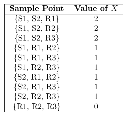
Hence, the random variable \(X\) can take the values \(0, 1, 2\) with the sample space completely enumerated.
Question: A coin is flipped until 3 heads in succession occur. List only those elements of the sample space that require 6 or fewer tosses. Is this a discrete sample space? Explain.
Solution:
We are to record sequences of coin tosses that result in the first occurrence of three successive heads (HHH) and require at most 6 tosses.
Step 1: Understand the stopping condition: We stop the experiment as soon as 3 consecutive heads occur. So we only include sequences that end with HHH and do not have HHH earlier in the sequence.
Step 2: List all such sequences of length $\leq 6$ that end with the first occurrence of HHH:
Length 3:
HHHLength 4:
THHHLength 5:
TTHHH,HTHH,HTTHHLength 6:
TTTHHH,THTHHH,HTTHHH,HHTTHH,HTHTHH
(The list can be extended exhaustively by generating all valid sequences of length $\leq 6$ that end with the HHH and have no earlier HHH. This process requires a state-based approach or tree traversal for accuracy.)
Step 3: Is the sample space discrete?
Yes, this is a discrete sample space because:
The outcomes (coin sequences) can be listed individually.
Each outcome corresponds to a finite sequence of tosses.
There are a countable number of possible outcomes even though the experiment could theoretically continue beyond 6 tosses.
Conclusion: The sample space consists of all sequences that end with the first appearance of 3 successive heads, and the total set is countable. Therefore, it is a discrete sample space.
Question: The shelf life, in days, for bottles of a certain prescribed medicine is a random variable having the density function \[ f(x) = \begin{cases} \frac{20,\!000}{(x+100)^3}, & x > 0 \\ 0, & \text{elsewhere} \end{cases} \] Find the probability that a bottle of this medicine will have a shelf life of (a) at least 200 days; (b) anywhere from 80 to 120 days.
Solution:
This is a continuous probability density function. To find probabilities, we integrate the density over the desired interval.
—
(a) Probability that shelf life is at least 200 days: We want \( P(X \geq 200) = \int_{200}^{\infty} \frac{20000}{(x+100)^3} dx \)
Let us make the substitution: Let \( u = x + 100 \Rightarrow du = dx \), when \( x = 200 \), \( u = 300 \)
\begin{align*} P(X \geq 300) &= \int_{300}^{\infty} \frac{20000}{u^3} \, du \\ &= 20000 \int_{300}^{\infty} u^{-3} \, du \\ &= 20000 \left[ \frac{u^{-2}}{-2} \right]_{300}^{\infty} \\ &= 20000 \left( 0 - \left( \frac{-1}{2 \cdot 300^2} \right) \right) \\ &= \frac{20000}{2 \cdot 300^2} \\ &= \frac{20000}{180000} \\ &= \frac{1}{9} \end{align*}
\[ \boxed{P(X \geq 200) = \frac{1}{9}} \]
—
(b) Probability that shelf life is between 80 and 120 days: We want \( P(80 \leq X \leq 120) = \int_{80}^{120} \frac{20000}{(x+100)^3} dx \)
Use substitution \( u = x + 100 \Rightarrow du = dx \) When \( x = 80 \), \( u = 180 \); When \( x = 120 \), \( u = 220 \)
\begin{align*} P(180 \leq X \leq 220) &= \int_{180}^{220} \frac{20000}{u^3} \, du \\ &= 20000 \int_{180}^{220} u^{-3} \, du \\ &= 20000 \left[ \frac{u^{-2}}{-2} \right]_{180}^{220} \\ &= 20000 \left( \frac{-1}{2 \cdot 220^2} + \frac{1}{2 \cdot 180^2} \right) \\ &= \frac{20000}{2} \left( \frac{1}{180^2} - \frac{1}{220^2} \right) \\ &= 10000 \left( \frac{1}{32400} - \frac{1}{48400} \right) \\ &= 10000 \left( \frac{48400 - 32400}{32400 \cdot 48400} \right) \\ &= 10000 \cdot \frac{16000}{1,\!568,\!160,\!000} \\ &= \frac{160,\!000,\!000}{1,\!568,\!160,\!000} \\ &= \boxed{\frac{10}{98.01} \approx 0.102} \end{align*} So, \[ \boxed{P(80 \leq X \leq 120) \approx 0.102} \]
Problem:
The total number of hours, measured in units of 100 hours, that a family runs a vacuum cleaner over a period of one year is a continuous random variable \( X \) with the density function:
\[ f(x) = \begin{cases} x, & 0 < x < 1 \\ 2 - x, & 1 \le x < 2 \\ 0, & \text{otherwise} \end{cases} \]
Find the probability that over a period of one year, a family runs their vacuum cleaner:
(a) less than 120 hours;
(b) between 50 and 100 hours.
Solution:
The given PDF \( f(x) \) is a piecewise function over the domain \( (0,2) \). Since \( x \) is in 100-hour units:
120 hours = 1.2 units
50 hours = 0.5 units
100 hours = 1 unit
(a) Probability that \( X < 1.2 \):
\[ P(X < 1.2) = \int_0^1 x \, dx + \int_1^{1.2} (2 - x) \, dx \]
First integral: \[ \int_0^1 x \, dx = \left[\frac{x^2}{2}\right]_0^1 = \frac{1}{2} \]
Second integral: \[ \int_1^{1.2} (2 - x) \, dx = \left[2x - \frac{x^2}{2}\right]_1^{1.2} = \left(2(1.2) - \frac{(1.2)^2}{2}\right) - \left(2(1) - \frac{(1)^2}{2}\right) \] \[ = (2.4 - 0.72) - (2 - 0.5) = 1.68 - 1.5 = 0.18 \]
So, \[ P(X < 1.2) = 0.5 + 0.18 = \boxed{0.68} \]
(b) Probability that \( 0.5 < X < 1 \):
This falls entirely in the first part of the PDF \( f(x) = x \):
\[ P(0.5 < X < 1) = \int_{0.5}^{1} x \, dx = \left[\frac{x^2}{2}\right]_{0.5}^1 = \frac{1}{2} - \frac{(0.5)^2}{2} = \frac{1}{2} - \frac{0.25}{2} = \frac{1}{2} - 0.125 = \boxed{0.375} \]
Problem:
The proportion of people who respond to a certain mails is a continuous random variable \( X \) that has the density function: \[ f(x) = \begin{cases} \dfrac{2(x+2)}{5}, & 0 < x < 1 \\ 0, & \text{otherwise} \end{cases} \]
(a) Show that \( P(0 < X < 1) = 1 \).
(b) Find the probability that more than \( \frac{1}{4} \) but less than \( \frac{1}{2} \) of the people respond.
Solution:
(a) We verify that the total probability over the range of the PDF is 1:
\[ P(0 < X < 1) = \int_0^1 \frac{2(x+2)}{5} \, dx = \frac{2}{5} \int_0^1 (x + 2) \, dx \] \[ = \frac{2}{5} \left[ \frac{x^2}{2} + 2x \right]_0^1 = \frac{2}{5} \left( \frac{1}{2} + 2 \right) = \frac{2}{5} \cdot \frac{5}{2} = 1 \]
Hence, the PDF is valid.
(b) We find the probability: \[ P\left( \frac{1}{4} < X < \frac{1}{2} \right) = \int_{1/4}^{1/2} \frac{2(x+2)}{5} \, dx = \frac{2}{5} \int_{1/4}^{1/2} (x + 2) \, dx \] \[ = \frac{2}{5} \left[ \frac{x^2}{2} + 2x \right]_{1/4}^{1/2} \]
Evaluating: \[ \left( \frac{1}{2} \right)^2/2 + 2 \cdot \frac{1}{2} = \frac{1}{8} + 1 = \frac{9}{8} \] \[ \left( \frac{1}{4} \right)^2/2 + 2 \cdot \frac{1}{4} = \frac{1}{32} + \frac{1}{2} = \frac{17}{32} \] \[ \Rightarrow \frac{9}{8} - \frac{17}{32} = \frac{36 - 17}{32} = \frac{19}{32} \] \[ \Rightarrow \frac{2}{5} \cdot \frac{19}{32} = \frac{38}{160} = \boxed{\frac{19}{80} = 0.2375} \]
Problem:
A continuous random variable \( X \) that can assume values between \( x = 2 \) and \( x = 5 \) has a density function given by:
\[ f(x) = \frac{2(1 + x)}{27}, \quad 2 \le x \le 5 \]
Find:
[(a)] \( P(X < 4) \)
[(b)] \( P(3 \le X < 4) \)
Solution:
(a) Compute \( P(X < 4) \):
\[ P(X < 4) = \int_{2}^{4} \frac{2(1 + x)}{27} \, dx = \frac{2}{27} \int_{2}^{4} (1 + x) \, dx \] \[ = \frac{2}{27} \left[ x + \frac{x^2}{2} \right]_2^4 = \frac{2}{27} \left( \left(4 + \frac{16}{2} \right) - \left(2 + \frac{4}{2} \right) \right) \] \[ = \frac{2}{27} \left( 4 + 8 - 2 - 2 \right) = \frac{2}{27} \cdot 8 = \frac{16}{27} \]
\[ \boxed{P(X < 4) = \frac{16}{27} \approx 0.5926} \]
(b) Compute \( P(3 \le X < 4) \):
\[ P(3 \le X < 4) = \int_{3}^{4} \frac{2(1 + x)}{27} \, dx = \frac{2}{27} \int_{3}^{4} (1 + x) \, dx \] \[ = \frac{2}{27} \left[ x + \frac{x^2}{2} \right]_3^4 = \frac{2}{27} \left( \left(4 + \frac{16}{2} \right) - \left(3 + \frac{9}{2} \right) \right) \] \[ = \frac{2}{27} \left( 4 + 8 - 3 - 4.5 \right) = \frac{2}{27} \cdot 4.5 = \frac{9}{27} = \frac{1}{3} \]
\[ \boxed{P(3 \le X < 4) = \frac{1}{3} \approx 0.3333} \]
Joint Probability Distributions
Let \(X\) and \(Y\) be discrete random variables. A function \(f(x, y)\) is called the joint probability distribution of \(X\) and \(Y\) if:
\(f(x, y) \geq 0\) for all \((x, y)\),
\(\sum_x \sum_y f(x, y) = 1\),
\(P(X = x, Y = y) = f(x, y)\)
For any region \(A\) in the \(xy\)-plane: \[ P[(X, Y) \in A] = \sum_{(x, y) \in A} f(x, y) \]
Problem:
Two ballpoint pens are selected at random from a box containing 3 blue, 2 red, and 3 green pens (8 pens total).
Let: \[ X = \text{Number of blue pens selected}, \quad Y = \text{Number of red pens selected} \]
(a) Find the joint probability mass function \(f(x, y)\). (b) Compute \(P(X + Y \leq 1)\)
Solution:
There are \({8 \choose 2} = 28\) possible ways to choose 2 pens from 8.
We list valid combinations of \((X, Y)\) where \(x + y \leq 2\), \(x \leq 2\), \(y \leq 2\), and \(x + y \leq 2\):
\((0,0)\): 2 green → \({3 \choose 2} = 3\)
\((1,0)\): 1 blue, 1 green → \(3 \times 3 = 9\)
\((0,1)\): 1 red, 1 green → \(2 \times 3 = 6\)
\((1,1)\): 1 blue, 1 red → \(3 \times 2 = 6\)
\((2,0)\): 2 blue → \({3 \choose 2} = 3\)
\((0,2)\): 2 red → \({2 \choose 2} = 1\)
So, joint pmf \(f(x,y)\) is:
\[ \begin{aligned} f(0,0) &= \frac{3}{28}, \quad f(1,0) = \frac{9}{28}, \quad f(0,1) = \frac{6}{28}, \\ f(1,1) &= \frac{6}{28}, \quad f(2,0) = \frac{3}{28}, \quad f(0,2) = \frac{1}{28} \end{aligned} \]
(b) \(P(X + Y \leq 1) = f(0,0) + f(1,0) + f(0,1) = \frac{3 + 9 + 6}{28} = \frac{18}{28} = \frac{9}{14}\)
Problem:
A fair coin is tossed 3 times. Let: \[ X = \text{Number of Heads}, \quad Y = \text{Number of Tails} \]
(a) Find the joint pmf \(f(x, y)\). (b) Find \(P(X = 2, Y = 1)\)
Solution:
All outcomes: HHH, HHT, HTH, THH, HTT, THT, TTH, TTT — total of 8 outcomes.
Count heads and tails in each: \[ \begin{aligned} &\text{HHH} \rightarrow (3,0) \\ &\text{HHT, HTH, THH} \rightarrow (2,1) \quad \text{(3 outcomes)} \\ &\text{HTT, THT, TTH} \rightarrow (1,2) \quad \text{(3 outcomes)} \\ &\text{TTT} \rightarrow (0,3) \end{aligned} \]
Thus, the joint pmf is:
\[ \begin{aligned} f(3,0) &= \frac{1}{8}, \\ f(2,1) &= \frac{3}{8}, \\ f(1,2) &= \frac{3}{8}, \\ f(0,3) &= \frac{1}{8} \end{aligned} \]
(b) \(P(X = 2, Y = 1) = f(2,1) = \frac{3}{8}\)
When $X$ and $Y$ are continuous random variables, their joint density function $f(x, y)$ defines a surface over the $xy$-plane. The probability that $(X, Y)$ lies in a region $A$ is equal to the volume under the surface $f(x, y)$ over that region.
Definition: The function $f(x, y)$ is a joint density function if:
$f(x, y) \geq 0$ for all $(x, y)$,
$\int_{-\infty}^{\infty} \int_{-\infty}^{\infty} f(x, y) \, dx \, dy = 1$,
$P[(X, Y) \in A] = \int\int_{A} f(x, y) \, dx \, dy$, for any region $A$ in the $xy$-plane.
Let $X$ and $Y$ be the proportion of time that a drive-in and a walk-in facility are in use, respectively. Their joint density function is:
\[ f(x, y) = \begin{cases} \frac{2}{5}(2x + 3y), & 0 \leq x \leq 1,\ 0 \leq y \leq 1, \\ 0, & \text{otherwise}. \end{cases} \]
(a) Verify that $f(x, y)$ is a valid joint density function:
\begin{align*} \iint_{\mathbb{R}^2} f(x, y) \, dy \, dx &= \int_0^1 \int_0^1 \frac{2}{5}(2x + 3y) \, dy \, dx \\ &= \int_0^1 \left[ \frac{2}{5} \left(2xy + \frac{3}{2} y^2 \right) \bigg|_0^1 \right] dx \\ &= \int_0^1 \frac{2}{5} \left(2x + \frac{3}{2} \right) dx \\ &= \frac{2}{5} \int_0^1 \left(2x + \frac{3}{2} \right) dx \\ &= \frac{2}{5} \left[ x^2 + \frac{3}{2}x \right]_0^1 \\ &= \frac{2}{5} \left(1 + \frac{3}{2} \right) = \frac{2}{5} \cdot \frac{5}{2} = 1 \end{align*}
So, the function satisfies the condition of total probability being 1.
(b) Find $P\left(0 < x < \frac{1}{2},\ \frac{1}{4} < y < \frac{1}{2}\right)$:
\begin{align*} P &= \int_0^{1/2} \int_{1/4}^{1/2} \frac{2}{5}(2x + 3y) \, dy \, dx \\ &= \int_0^{1/2} \left[ \frac{2}{5} \left(2xy + \frac{3}{2} y^2 \right) \bigg|_{1/4}^{1/2} \right] dx \\ &= \int_0^{1/2} \frac{2}{5} \left(2x \cdot \left(\frac{1}{2} - \frac{1}{4} \right) + \frac{3}{2} \left( \left(\frac{1}{2}\right)^2 - \left(\frac{1}{4}\right)^2 \right) \right) dx \\ &= \int_0^{1/2} \frac{2}{5} \left( \frac{x}{2} + \frac{3}{2} \cdot \left( \frac{1}{4} - \frac{1}{16} \right) \right) dx \\ &= \int_0^{1/2} \frac{2}{5} \left( \frac{x}{2} + \frac{3}{2} \cdot \frac{3}{16} \right) dx \\ &= \int_0^{1/2} \frac{2}{5} \left( \frac{x}{2} + \frac{9}{32} \right) dx \\ &= \frac{2}{5} \left[ \frac{x^2}{4} + \frac{9x}{32} \right]_0^{1/2} \\ &= \frac{2}{5} \left( \frac{1}{16} + \frac{9}{64} \right) = \frac{2}{5} \cdot \frac{13}{64} = \frac{26}{320} = \frac{13}{160} \end{align*}
Let $f(x, y) = 6xy$ for $0 < x < 1$, $0 < y < 1$ and 0 elsewhere.
Check $f(x, y)$ is a valid joint density function?
Solution:
We compute:
\[ \int_0^1 \int_0^1 6xy \, dy \, dx = \int_0^1 6x \left[ \frac{y^2}{2} \right]_0^1 dx = \int_0^1 6x \cdot \frac{1}{2} dx = 3 \int_0^1 x \, dx = 3 \cdot \frac{1}{2} = \boxed{1.5}. \]
So, it's not a valid joint density function.
Marginal Probability Distributions
Definition: Given the joint probability distribution \( f(x, y) \) of the discrete random variables \( X \) and \( Y \), the probability distribution \( g(x) \) of \( X \) alone is obtained by summing \( f(x, y) \) over the values of \( y \), and the probability distribution \( h(y) \) of \( Y \) alone is obtained by summing \( f(x, y) \) over the values of \( x \). These are called the marginal distributions of \( X \) and \( Y \), respectively.
For the discrete case: \[ g(x) = \sum_y f(x, y), \quad h(y) = \sum_x f(x, y) \]
For the continuous case: \[ g(x) = \int_{-\infty}^{\infty} f(x, y) \, dy, \quad h(y) = \int_{-\infty}^{\infty} f(x, y) \, dx \]
The term marginal is used because these are the totals of the respective rows and columns in a joint probability table.
Example: Show that the column and row totals of Table given give the marginal distributions of \( X \) and \( Y \). \[ \begin{array}{c|ccc|c} f(x,y) & x=0 & x=1 & x=2 & \text{Row Totals} \\ y=0 & \frac{3}{28} & \frac{9}{28} & \frac{3}{28} & \frac{15}{28} \\ y=1 & \frac{3}{14} & \frac{3}{14} & 0 & \frac{3}{7} \\ y=2 & \frac{1}{28} & 0 & 0 & \frac{1}{28} \\ \text{Column Totals} & \frac{5}{14} & \frac{15}{28} & \frac{3}{28} & 1 \end{array} \]
Solution: Using the values from Table :
\[ \begin{aligned} g(0) &= f(0,0) + f(0,1) + f(0,2) = \frac{3}{28} + \frac{6}{28} + \frac{1}{28} = \frac{10}{28} = \frac{5}{14}, \\ g(1) &= f(1,0) + f(1,1) + f(1,2) = \frac{9}{28} + \frac{6}{28} + 0 = \frac{15}{28}, \\ g(2) &= f(2,0) + f(2,1) + f(2,2) = \frac{3}{28} + 0 + 0 = \frac{3}{28}. \end{aligned} \]
Similarly, for \( Y \):
.+- \[ \begin{aligned} h(0) &= f(0,0) + f(1,0) + f(2,0) = \frac{3}{28} + \frac{9}{28} + \frac{3}{28} = \frac{15}{28}, \\ h(1) &= f(0,1) + f(1,1) + f(2,1) = \frac{6}{28} + \frac{6}{28} + 0 = \frac{12}{28} = \frac{3}{7}, \\ h(2) &= f(0,2) + f(1,2) + f(2,2) = \frac{1}{28} + 0 + 0 = \frac{1}{28}. \end{aligned} \]
Marginal Distributions in Table Form:
\[ \begin{array}{c|ccc} x & 0 & 1 & 2 \\ g(x) & \frac{5}{14} & \frac{15}{28} & \frac{3}{28} \end{array} \qquad \begin{array}{c|ccc} y & 0 & 1 & 2 \\ h(y) & \frac{15}{28} & \frac{3}{7} & \frac{1}{28} \end{array} \]
Definition: For continuous random variables \( X \) and \( Y \) with joint probability density function \( f(x, y) \), the marginal distribution of \( X \) is: \[ g(x) = \int_{-\infty}^{\infty} f(x, y) \, dy \] and the marginal distribution of \( Y \) is: \[ h(y) = \int_{-\infty}^{\infty} f(x, y) \, dx \]
Example: Suppose the joint probability density function of \( X \) and \( Y \) is given by \[ f(x, y) = \begin{cases} 6xy & \text{if } 0 < x < 1, \ 0 < y < 1 \\ 0 & \text{otherwise} \end{cases} \]
(a) Find the marginal density function of \( X \), \( g(x) \). (b) Find the marginal density function of \( Y \), \( h(y) \).
Solution:
(a) Marginal density of \( X \): \[ g(x) = \int_0^1 6xy \, dy = 6x \int_0^1 y \, dy = 6x \cdot \left[\frac{y^2}{2}\right]_0^1 = 6x \cdot \frac{1}{2} = 3x \] So, \[ g(x) = \begin{cases} 3x & \text{if } 0 < x < 1 \\ 0 & \text{otherwise} \end{cases} \]
(b) Marginal density of \( Y \): \[ h(y) = \int_0^1 6xy \, dx = 6y \int_0^1 x \, dx = 6y \cdot \left[\frac{x^2}{2}\right]_0^1 = 6y \cdot \frac{1}{2} = 3y \] So, \[ h(y) = \begin{cases} 3y & \text{if } 0 < y < 1 \\ 0 & \text{otherwise} \end{cases} \]
Conditional Probability Distributions
Let \( X \) and \( Y \) be discrete random variables. The conditional distribution of the random variable \( Y \) given that \( X = x \) is defined as: \[ P(Y = y \mid X = x) = \frac{P(X = x, Y = y)}{P(X = x)}, \quad \text{provided } P(X = x) > 0. \]
Similarly, the conditional distribution of \( X \) given that \( Y = y \) is: \[ P(X = x \mid Y = y) = \frac{P(X = x, Y = y)}{P(Y = y)}, \quad \text{provided } P(Y = y) > 0. \]
To compute the probability that \( X \) lies between \( a \) and \( b \) given \( Y = y \), we sum: \[ P(a < X < b \mid Y = y) = \sum_{a < x < b} P(X = x \mid Y = y). \]
Let \( X \) and \( Y \) be continuous random variables with joint probability density function \( f(x, y) \). The conditional distribution of \( Y \) given that \( X = x \) is: \[ f(y \mid x) = \frac{f(x, y)}{g(x)}, \quad \text{where } g(x) = \int_{-\infty}^{\infty} f(x, y) \, dy, \quad \text{provided } g(x) > 0. \]
Similarly, the conditional distribution of \( X \) given that \( Y = y \) is: \[ f(x \mid y) = \frac{f(x, y)}{h(y)}, \quad \text{where } h(y) = \int_{-\infty}^{\infty} f(x, y) \, dx, \quad \text{provided } h(y) > 0. \]
To find the probability that \( X \) lies between \( a \) and \( b \) given \( Y = y \), we compute: \[ P(a < X < b \mid Y = y) = \int_a^b f(x \mid y) \, dx. \]
A fair 6-sided die is rolled twice. Let \( X \) be the outcome of the first roll and \( Y \) be the sum of both rolls. Find \( P(X = 3 \mid Y = 7) \).
Solution:
Total outcomes where \( Y = 7 \): \[ \begin{aligned} (X, Y - X) &= (1,6), (2,5), (3,4), \\ &\quad (4,3), (5,2), (6,1) \\ &\Rightarrow 6 \text{ outcomes} \\ \text{Out of these, only one has } X &= 3 \Rightarrow (3,4) \end{aligned} \] \[ P(X = 3 \mid Y = 7) = \frac{1}{6} \]
Let \( X \) and \( Y \) have joint PDF: \[ f(x, y) = \begin{cases} 8xy, & 0 < x < 1,\ 0 < y < x \\ 0, & \text{otherwise} \end{cases} \] Find the conditional density \( f(y \mid x) \).
Solution:
Marginal of \( X \): \[ f_X(x) = \int_0^x 8xy\, dy = 8x \cdot \left[\frac{y^2}{2}\right]_0^x = 4x^3 \]
So, conditional density: \[ f(y \mid x) = \frac{f(x, y)}{f_X(x)} = \frac{8xy}{4x^3} = \frac{2y}{x^2}, \quad 0 < y < x \]
Discrete Random Variable Probability Rules
|}
Rule 1: $P(X \le a)$
Formula: $P(X \le a) = F(a)$
Example: $P(X \le 2) = F(2) = P(X=0)+P(X=1)+P(X=2)=0.875$
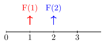
Visual:

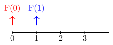
Rule 2: $P(X < a)$
Formula: $P(X < a) = F(a-1)$
Example: $P(X < 2) = F(1) = P(X=0)+P(X=1)=0.5$
Visual:
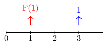
Rule 3: $P(X > a)$
Formula: $P(X > a) = 1 - F(a)$
Example: $P(X>1) = 1 - F(1) = 0.5$
Visual:
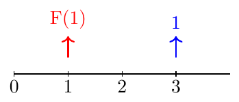
Rule 4: $P(X \ge a)$
Formula: $P(X \ge a) = 1 - F(a-1)$
Example: $P(X \ge 2) = 1 - F(1) = 0.5$
Visual:
Rule 5: $P(a \le X \le b)$
Formula: $P(a \le X \le b) = F(b)-F(a-1)$
Example: $P(1 \le X \le 2) = F(2)-F(0)=0.75$
Visual:
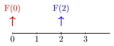
Rule 6: $P(a < X \le b)$
Formula: $P(a < X \le b) = F(b)-F(a)$
Example: $P(1 < X \le 2) = F(2)-F(1)=0.375$
Visual:
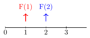
Rule 7: $P(a \le X < b)$
Formula: $P(a \le X < b) = F(b-1)-F(a-1)$
Example: $P(1 \le X < 3) = F(2)-F(0)=0.75$
Visual:
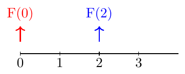
Rule 8: $P(a < X < b)$
Formula: $P(a < X < b) = F(b-1)-F(a)$
Example: $P(0 < X < 3) = F(2)-F(0)=0.75$
Visual:
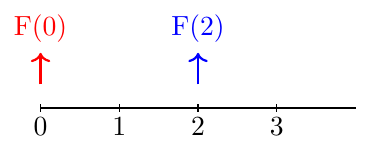
Rule 9: $P(X = a)$
Formula: $P(X = a) = F(a)-F(a-1)$
Example: $P(X=2) = F(2)-F(1)=0.375$
Visual:
Continuous Random Variable Probability Rules
|}
Rule 1: CDF at a point
\[
F(a) = P(X \le a) = P(X < a)
\]
In continuous case, the probability at a single point is zero.
So whether we write $X \le a$ or $X < a$, both mean the same.
Formally: \[ P(X = a) = \lim_{\epsilon \to 0^+} P(a \le X \le a+\epsilon) = 0 \]
Rule 2: Right tail probability
\[
P(X > a) = 1 - F(a)
\]
$F(a)$ already includes all probability up to $a$.
Since the entire distribution sums to $1$, the remaining area to the right is $1 - F(a)$.
Geometrically: probability under density curve to the right of $a$.
Rule 3: Interval probability
\[
P(a < X < b) = P(a \le X \le b) = F(b) - F(a)
\]
$F(b)$ counts probability up to $b$.
$F(a)$ counts probability up to $a$.
Subtraction gives probability between $a$ and $b$.
Since point probability is zero, choice of strict/weak inequalities doesn’t matter.