Chapter 8 of 8

Central Limit Theorem and Confidence Intervals

The Central Limit Theorem

Central Limit Theorem (CLT) Summary

Statement: If $ X_1, X_2, ..., X_n $ are independent and identically distributed (i.i.d.) random variables with mean $ \mu $ and standard deviation $ \sigma $, then for large $ n $, the sampling distribution of the sample mean $ \bar{X} $ approximates a normal distribution, regardless of the original distribution.

\[ \bar{X} \sim N\left(\mu, \frac{\sigma}{\sqrt{n}}\right) \]

Z-Score Formula (when population standard deviation is known): \[ Z = \frac{\bar{X} - \mu}{\sigma/\sqrt{n}} \]

T-Score Formula (when population standard deviation is unknown): \[ t = \frac{\bar{X} - \mu}{s/\sqrt{n}}, \quad \text{df} = n - 1 \]

Conditions to Use CLT:

Sample size $ n \geq 30 $ (for non-normal populations).
Random sampling.
Independence of observations.

Tip to Identify: Keywords like "average", "sample mean", "distribution of sample means", "approximate normal", "large sample size" suggest CLT usage.

Examples

Example 1: Average Weight (CLT Application)

The average weight of a mango is 250 grams with a standard deviation of 40 grams. If a sample of 64 mangoes is taken, what is the probability that their average weight is less than 245 grams?

Solution:
Here: $ \mu = 250 $, $ \sigma = 40 $, $ n = 64 $, $ \bar{X} = 245 $

\[ Z = \frac{245 - 250}{40/\sqrt{64}} = \frac{-5}{5} = -1 \]

Using standard normal table, $ P(Z < -1) = 0.1587 $

Answer: Probability is approximately $ \boxed{0.1587} $

Example 2: T-distribution for Small Sample

The IQ of students has unknown population standard deviation. A sample of 25 students has a mean IQ of 105 with sample standard deviation 10. What is the probability that the true mean is less than 108?

Solution:
Given: $ \bar{X} = 105 $, $ s = 10 $, $ n = 25 $, $ \mu = 108 $

\[ t = \frac{105 - 108}{10/\sqrt{25}} = \frac{-3}{2} = -1.5, \quad df = 24 \]

Using t-table, $ P(t < -1.5) \approx 0.07 $

Answer: Probability is approximately $ \boxed{0.07} $

Example 3: Average Height

The average height of a species of plant is 120 cm with $ \sigma = 15 $ cm. What is the probability that a sample of 36 plants has a mean height between 117 cm and 123 cm?

Solution:

\[ Z_1 = \frac{117 - 120}{15/\sqrt{36}} = \frac{-3}{2.5} = -1.2,\quad Z_2 = \frac{123 - 120}{15/\sqrt{36}} = 1.2 \]

Using standard normal table: \[ P(-1.2 < Z < 1.2) = 2 \times P(Z < 1.2) - 1 = 2 \times 0.8849 - 1 = 0.7698 \]

Answer: Probability is approximately $ \boxed{0.7698} $

Example 4: Machine Producing Screws

A machine produces screws with a mean weight of 5g and standard deviation 0.2g. What is the probability that a sample of 100 screws has a mean weight greater than 5.03g?

Solution: \[ Z = \frac{5.03 - 5}{0.2/\sqrt{100}} = \frac{0.03}{0.02} = 1.5 \] \[ P(Z > 1.5) = 1 - 0.9332 = 0.0668 \]

Answer: Probability is approximately $ \boxed{0.0668} $

Example 5: Sample Mean in Exams

Exam scores are normally distributed with mean 70 and $ \sigma = 10 $. What's the probability that a sample of 49 students scores above 72 on average?

Solution: \[ Z = \frac{72 - 70}{10/\sqrt{49}} = \frac{2}{1.43} \approx 1.4 \] \[ P(Z > 1.4) = 1 - 0.9192 = 0.0808 \]

Answer: Probability is approximately $ \boxed{0.0808} $

Confidence Intervals

Introduction to Confidence Interval

A Confidence Interval (CI) is a range of values, derived from sample statistics, that is likely to contain the value of an unknown population parameter. It is associated with a confidence level, which quantifies the level of confidence that the parameter lies within the interval.

For example, a 95% confidence interval for the population mean suggests that if we were to take 100 different samples and compute a CI for each, approximately 95 of those intervals would contain the true population mean.

Alpha ($\alpha$) and Confidence Level

Alpha ($\alpha$) represents the probability of rejecting the true parameter. It is given by: \[ \alpha = 1 - \text{Confidence Level} \] For example, if the confidence level is 95%, then $\alpha = 0.05$.

In a two-tailed test, $\alpha/2$ is the area in each tail.

Degrees of Freedom

The degrees of freedom (df) refer to the number of values in the final calculation of a statistic that are free to vary. For estimating the population mean using sample variance, the degrees of freedom are: \[ df = n - 1 \] where $n$ is the sample size.

Confidence Interval for Population Mean (Known Standard Deviation - Z Test)

Formula: \[ CI = \bar{x} \pm z_{\alpha/2} \cdot \frac{\sigma}{\sqrt{n}} \]

$\bar{x}$ = sample mean
$\sigma$ = population standard deviation
$n$ = sample size
$z_{\alpha/2}$ = critical value from standard normal distribution

Confidence Interval for Population Mean (Unknown Standard Deviation - T Test)

Formula: \[ CI = \bar{x} \pm t_{\alpha/2, df} \cdot \frac{s}{\sqrt{n}} \]

$s$ = sample standard deviation
$t_{\alpha/2, df}$ = critical value from t-distribution with $df = n - 1$

Confidence Interval for Population Variance (Chi-Squared Test)

Formula: \[ \left( \frac{(n-1)s^2}{\chi^2_{\alpha/2}}, \frac{(n-1)s^2}{\chi^2_{1 - \alpha/2}} \right) \]

$\chi^2$ = critical value from chi-square distribution
$s^2$ = sample variance
$n$ = sample size

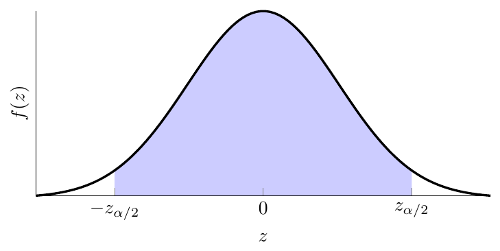
Confidence Level and Alpha Visualization

The shaded area represents the 95% confidence region. The tails (unshaded) represent $\alpha/2 = 0.025$ each.