Continuous Probability Distributions
Uniform Distribution
A continuous uniform distribution is a probability distribution in which all values between two specified limits (\(a\) and \(b\)) are equally likely. The probability is uniformly spread over the interval \([a, b]\).
Probability Density Function (PDF): \[ f(x) = \begin{cases} \frac{1}{b-a}, & a \leq x \leq b \\ 0, & \text{otherwise} \end{cases} \]
Mean (Expected Value): \[ E(X) = \frac{a + b}{2} \]
Variance: \[ \text{Var}(X) = \frac{(b - a)^2}{12} \]
Cumulative Distribution Function (CDF): \[ F(x) = \begin{cases} 0, & x < a \\ \frac{x - a}{b - a}, & a \leq x \leq b \\ 1, & x > b \end{cases} \]
The variable is continuous and can take any real value within a specified range.
Every value between \(a\) and \(b\) is equally likely.
The problem may mention a flat or constant probability density.
Usually used for time, distance, or measurement-based outcomes.
Keywords to look for:
“equally likely between a and b”
“randomly chosen between two continuous values”
“uniformly distributed over an interval”
Examples
A commuter arriving at a bus stop finds that the time between successive buss is uniformly distributed between 0 and 20 minutes. Let \(X\) be the waiting time (in minutes) from the commuter's arrival until the next bus. Find:
[i.] The PDF of \(X\).
[ii.] The probability that the commuter waits more than 7 minutes.
[iii.] The expected waiting time and the variance.
Solution:
Since interarrival times are uniform on \([0,20]\), we have \(X\sim U(0,20)\).
[i.] The PDF of a continuous uniform on \([a,b]\) is \[ f_X(x)=\begin{cases} \dfrac{1}{b-a}, & a\le x\le b,\\[4pt] 0, & \text{otherwise.} \end{cases} \] Here \(a=0,b=20\), so \[ f_X(x)=\frac{1}{20},\quad 0\le x\le 20. \]
[ii.] For \(X\sim U(0,20)\), \[ P(X>7)=\frac{b-7}{b-a}=\frac{20-7}{20-0}=\frac{13}{20}=0.65. \] (Alternatively integrate: \(\int_{7}^{20}\tfrac{1}{20}\,dx=\tfrac{13}{20}\).)
[iii.] The mean and variance of \(U(a,b)\) are \[ E[X]=\frac{a+b}{2},\qquad \mathrm{Var}(X)=\frac{(b-a)^2}{12}. \] Thus \[ E[X]=\frac{0+20}{2}=10,\qquad \mathrm{Var}(X)=\frac{20^2}{12}=\frac{400}{12}=\frac{100}{3}\approx 33.3333. \]
A laboratory thermostat produces temperatures uniformly between \(10^\circ\)C and \(50^\circ\)C during a calibration process. Let \(X\) denote the recorded temperature. Compute:
[i.] The mean and variance of \(X\).
[ii.] The probability that \(X<30^\circ\)C.
Solution:
Here \(X\sim U(10,50)\) with \(a=10\), \(b=50\).
[i.] Mean: \[ E[X]=\frac{a+b}{2}=\frac{10+50}{2}=30. \] Variance: \[ \mathrm{Var}(X)=\frac{(b-a)^2}{12}=\frac{(50-10)^2}{12}=\frac{40^2}{12}=\frac{1600}{12}=\frac{400}{3}\approx 133.3333. \]
[ii.] Since the distribution is uniform, \[ P(X<30)=\frac{30-10}{50-10}=\frac{20}{40}=\frac{1}{2}=0.5. \] (Equivalently, integrate \(f_X(x)=1/40\) from \(10\) to \(30\): \(\int_{10}^{30}\tfrac{1}{40}\,dx=\tfrac{20}{40}\).)
A customer support call lasts uniformly between 2 and 12 minutes. Let \(X\) denote the call duration (minutes). Find the probability that a randomly selected call lasts between 4 and 9 minutes. Also give the PDF and expected call duration.
Solution:
\(X\sim U(2,12)\) so \(a=2\), \(b=12\).
PDF: \[ f_X(x)=\frac{1}{b-a}=\frac{1}{10},\quad 2\le x\le 12. \]
Probability: \[ P(4\le X\le 9)=\frac{9-4}{12-2}=\frac{5}{10}=0.5. \] (Integration: \(\int_4^9 \tfrac{1}{10}\,dx=\tfrac{5}{10}\).)
Expected value: \[ E[X]=\frac{2+12}{2}=7\ \text{minutes}. \] (Variance for completeness: \(\mathrm{Var}(X)=\dfrac{10^2}{12}=\dfrac{100}{12}=\dfrac{25}{3}\approx 8.3333\).)
Let \(X \sim U(0,4)\) and \(Y \sim U(0,6)\), independent random variables. Find:
[i.] The probability that \(X + Y < 5\).
[ii.] The probability that \(X > Y\).
Solution: Both \(X\) and \(Y\) are uniform on \([0,4]\times[0,6]\), so total area \(=24\).
(i) \(P(X+Y<5)\):
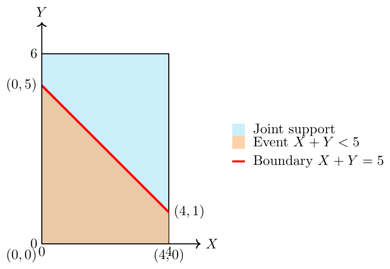
Area \(=\int_0^4 (5-x)\,dx =12 \Rightarrow P(X+Y<5)=\tfrac{12}{24}=\tfrac12.\)
(ii) \(P(X>Y)\):
Favourable region: triangle below \(x=4\) and above \(y=x\). Area \(=\int_0^4(4-y)\,dy=8 \Rightarrow P(X>Y)=\tfrac{8}{24}=\tfrac13.\)
Final answers: (i) \(\tfrac{1}{2}\), (ii) \(\tfrac{1}{3}\).
Let \(X\) be uniformly distributed on \([-2,\,5]\). Find the cumulative distribution function \(F_X(x)\). Solution:
For \(X\sim U(a,b)\) with \(a=-2\), \(b=5\), the CDF is \[ F_X(x)=\begin{cases} 0, & x<a=-2,\\[4pt] \dfrac{x-a}{b-a}=\dfrac{x+2}{7}, & -2\le x\le 5,\\[8pt] 1, & x>b=5. \end{cases} \] This piecewise formula gives, for example, \(F_X(0)=\dfrac{0+2}{7}=\dfrac{2}{7}\).
Median: For a continuous uniform the median equals the mean: \[ \text{median}=\frac{a+b}{2}=\frac{-2+5}{2}=\frac{3}{2}=1.5. \]
Exponential Distribution
The Exponential Distribution is a continuous probability distribution used to model the time between successive events in a Poisson process. It is memoryless, meaning the probability of an event occurring in the future is independent of the past.
Probability Density Function (PDF): \[ f(x; \lambda) = \lambda e^{-\lambda x}, \quad x \ge 0, \lambda > 0 \]
Cumulative Distribution Function (CDF): \[ F(x) = 1 - e^{-\lambda x} \]
Mean (Expected Value): \[ E(X) = \frac{1}{\lambda} \]
Variance: \[ Var(X) = \frac{1}{\lambda^2} \]
Memoryless Property: \[ P(X > s + t \mid X > s) = P(X > t) \]
Look for the following keywords in the problem statement:
"Time between arrivals"
"Waiting time until the next event"
"Lifetimes of devices or components"
"Memoryless property"
Events that happen independently and continuously over time
Such problems are often tied to Poisson processes, where the inter-arrival times are exponentially distributed.
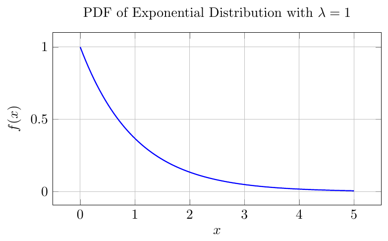
The PDF is highest at $x = 0$ and decreases exponentially.
Examples
The average time between calls at a call center is 3 minutes. What is the probability that the next call comes in more than 5 minutes?
Solution: $\lambda = \frac{1}{3}$.
We use: $P(X > 5) = e^{-\lambda x} = e^{-5/3} \approx 0.1889$.
The time to failure of a light bulb follows an exponential distribution with $\lambda = 0.02$. What is the expected life of the bulb?
Solution: $E(X) = \frac{1}{\lambda} = \frac{1}{0.02} = 50$ hours.
If a system fails with a mean time of 10 hours, find the probability that it fails before 4 hours.
Solution: $\lambda = 1/10$.
$P(X < 4) = 1 - e^{-\lambda x} = 1 - e^{-0.4} \approx 0.3297$.
A machine breaks down on average every 15 days. What is the variance in the time between breakdowns?
Solution: $\lambda = 1/15$, so: $Var(X) = \frac{1}{\lambda^2} = 225$ days².
A component lasts more than 8 years with probability 0.2. What is the failure rate $\lambda$?
Solution: $P(X > 8) = e^{-\lambda \cdot 8} = 0.2$.
Taking $\ln$ on both sides: $-8\lambda = \ln(0.2) \Rightarrow \lambda = -\frac{\ln(0.2)}{8} \approx 0.2012$.
Normal Distribution and Standard Normal
The Normal Distribution is a continuous probability distribution that is symmetric about its mean. It models many natural phenomena such as height, test scores, and measurement errors.
Probability Density Function (PDF): \[ f(x) = \frac{1}{\sigma \sqrt{2\pi}} e^{ -\frac{(x - \mu)^2}{2\sigma^2} } \]
Where:
$\mu$ = mean
$\sigma$ = standard deviation
$x$ = continuous random variable
Properties:
Symmetric about the mean
Mean = Median = Mode
Total area under the curve = 1
Empirical Rule:
68% data within 1$\sigma$
95% data within 2$\sigma$
99.7% data within 3$\sigma$
Graph of Normal Distribution
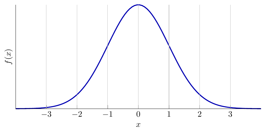
Standard Normal Curve (Mean = 0, Std. Dev = 1)
Tips to Identify Normal Distribution Problems
A problem likely involves a Normal Distribution if:
It involves continuous data (e.g., heights, weights, time).
You are given mean and standard deviation.
The data is symmetric or bell-shaped.
It mentions that data follows a "normal distribution" or "Gaussian distribution".
It asks for probability between two values or more/less than a certain value.
It involves a standardization step using Z-scores.
Standard Normal Distribution
The Standard Normal Distribution is a special case of the Normal Distribution where the mean ($\mu$) is 0 and the standard deviation ($\sigma$) is 1.
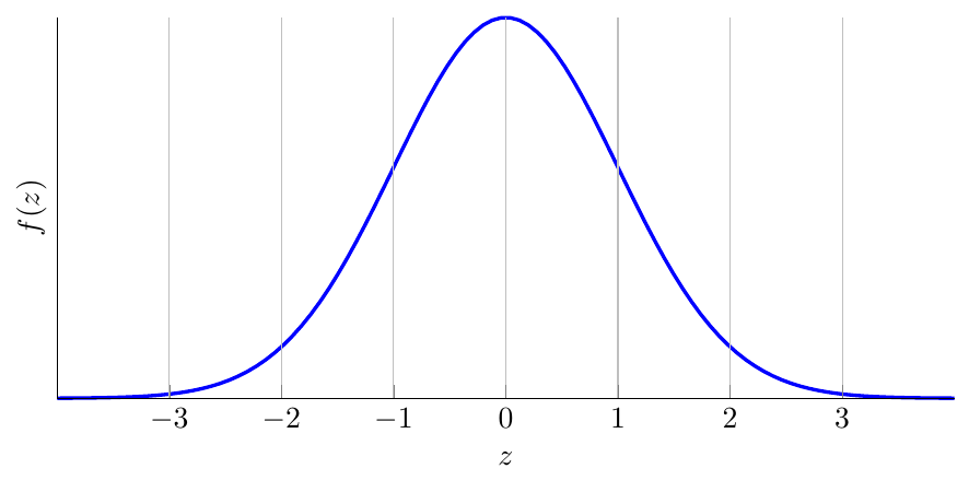
A random variable $Z$ follows a standard normal distribution if it has the following probability density function (pdf): \[ f(z) = \frac{1}{\sqrt{2\pi}} e^{-z^2/2}, \quad -\infty < z < \infty \]
This distribution is symmetric about $z=0$.
To convert a normal variable $X \sim N(\mu, \sigma^2)$ to a standard normal variable $Z$, we use: \[ Z = \frac{X - \mu}{\sigma} \] The Z-score tells us how many standard deviations a value is from the mean.
Use the Standard Normal Distribution when:
You are dealing with a normally distributed variable and have been given the mean and standard deviation.
You are asked to compute probabilities or quantiles using Z-scores.
The problem involves symmetry around the mean.
Values are standardized (i.e., Z-scores are used).
Examples
The weights of apples in an orchard are normally distributed with a mean of 150 g and a standard deviation of 12 g. What is the probability that a randomly chosen apple weighs more than 165 g?
\[ Z = \frac{165 - 150}{12} = 1.25 \] \[ P(X > 165) = P(Z > 1.25) = 1 - 0.8944 = 0.1056 \] Answer: 10.56%
The lifespan of LED bulbs follows a normal distribution with mean 2000 hours and standard deviation 200 hours. What is the probability that a bulb lasts between 1800 and 2200 hours?
\[ Z_1 = \frac{1800 - 2000}{200} = -1,\quad Z_2 = \frac{2200 - 2000}{200} = 1 \] \[ P(1800 < X < 2200) = P(-1 < Z < 1) = 0.8413 - 0.1587 = 0.6826 \] Answer: 68.26%
The volume of milk in a carton is normally distributed with mean 1000 ml and standard deviation 8 ml. What percentage of cartons will contain more than 1015 ml?
\[ Z = \frac{1015 - 1000}{8} = 1.875 \Rightarrow P(Z > 1.875) = 1 - 0.9699 = 0.0301 \] Answer: 3.01%
Let $X \sim N(60, 16)$. Find the value $x$ such that $P(X < x) = 0.975$.
From Z-tables, $P(Z < 1.96) = 0.975$ \[ x = \mu + Z\sigma = 60 + 1.96 \cdot 4 = 60 + 7.84 = 67.84 \] Answer: 67.84
The exam scores in a statistics class are normally distributed with mean 70 and standard deviation 6. What is the probability that a student scores between 65 and 80?
\[ Z_1 = \frac{65 - 70}{6} = -0.83,\quad Z_2 = \frac{80 - 70}{6} = 1.67 \Rightarrow P = P(-0.83 < Z < 1.67) \] \[ = 0.9525 - 0.2033 = 0.7492 \] Answer: 74.92%
If $X \sim N(45, 9)$, find $P(42 < X < 50)$.
\[ Z_1 = \frac{42 - 45}{3} = -1,\quad Z_2 = \frac{50 - 45}{3} = 1.67 \] \[ P = P(-1 < Z < 1.67) = 0.9525 - 0.1587 = 0.7938 \] Answer: 79.38%
Find $x$ such that $P(X < x) = 0.20$ for $X \sim N(100, 25)$.
\[ P(Z < z) = 0.20 \Rightarrow z = -0.84 \] \[ x = \mu + z\sigma = 100 - 0.84 \cdot 5 = 95.8 \] Answer: 95.8
$X \sim N(500, 100^2)$. Find $P(X > 650)$.
\[ Z = \frac{650 - 500}{100} = 1.5 \Rightarrow P(Z > 1.5) = 1 - 0.9332 = 0.0668 \] Answer: 6.68%
For $X \sim N(0,1)$, find $P(|X| < 1.5)$.
\[ P(|X| < 1.5) = P(-1.5 < X < 1.5) = 0.9332 - 0.0668 = 0.8664 \] Answer: 86.64%
The battery life of a smartphone is normally distributed with mean 8 hours and standard deviation 1.2 hours. What is the probability that a phone lasts more than 10 hours?
\[ Z = \frac{10 - 8}{1.2} = 1.67 \Rightarrow P(Z > 1.67) = 1 - 0.9525 = 0.0475 \] Answer: 4.75%
t-Distribution
The Student's t-distribution is a probability distribution used when we want to estimate population parameters, particularly the mean, from a small sample, or when the population standard deviation is unknown.
Key Points:
It is symmetric and bell-shaped like the normal distribution.
It has heavier tails than the normal distribution, which accounts for more variability in small samples.
As the sample size increases, the t-distribution approaches the standard normal distribution.
Degrees of Freedom (df): - For a sample of size $n$, df = $n - 1$. - It reflects the number of independent values that can vary in your calculation.
Uses:
One-sample t-test: Compare a sample mean to a population mean.
Two-sample t-test: Compare the means of two independent samples.
Paired t-test: Compare means from two related samples.
Confidence intervals: Estimate population mean when standard deviation is unknown.
Examples
A sample of 12 students has an average test score of 78, with a sample standard deviation of 5. Test if this differs from the population mean of 75 using a t-test.
\[ t = \frac{\bar{x} - \mu}{s/\sqrt{n}} = \frac{78 - 75}{5/\sqrt{12}} \approx 2.08 \]
Degrees of freedom: $n - 1 = 11$. Compare $t$ with the critical value for df = 11 at $\alpha = 0.05$. Conclusion: $t > t_{0.05,11}$ → significant difference.
A dietitian wants to check if the average weight loss of a sample of 10 people differs from 3 kg. Given: $\bar{x}=2.5$, $s=0.8$.
\[ t = \frac{2.5 - 3}{0.8 / \sqrt{10}} \approx -1.98 \]
Degrees of freedom: $9$. Conclusion: Compare with critical $t$ for df = 9.
A company tests 15 batteries with mean lifetime 520 hours and sample standard deviation 25 hours. Population mean = 500 hours. Find the $t$-score.
\[ t = \frac{520 - 500}{25 / \sqrt{15}} \approx 3.10 \]
Degrees of freedom: $14$. Conclusion: $t > t_{0.05,14}$ → significant.
A class of 8 students has an average height of 170 cm and a sample standard deviation of 6 cm. Test if the mean differs significantly from 165 cm.
\[ t = \frac{170 - 165}{6 / \sqrt{8}} \approx 2.36 \]
Degrees of freedom: $7$. Conclusion: Compare with critical $t_{0.05,7}$ → significant.
A farmer measures the yield of 20 fields. Sample mean = 50 tons, $s=8$ tons, and population mean = 47 tons. Find the $t$-score.
\[ t = \frac{50 - 47}{8 / \sqrt{20}} \approx 1.68 \]
Degrees of freedom: $19$. Conclusion: Compare with critical $t_{0.05,19}$.
Chi-Squared Distribution
The Chi-Square ($\chi^2$) distribution is a continuous distribution commonly used to analyze variance and categorical data.
Key Points:
Skewed to the right, especially for small degrees of freedom.
Becomes more symmetric as df increases, approaching normality.
Degrees of freedom depend on sample size and the number of constraints (e.g., df = n - 1 for variance tests).
Uses:
Goodness-of-fit tests.
Test of independence in contingency tables.
Confidence intervals for variance of a normally distributed population.
Part of ANOVA test statistics.
Examples
A sample of 10 machines has variance 16. Test if the population variance is 9 using a chi-square test.
\[ \chi^2 = \frac{(n-1)s^2}{\sigma^2} = \frac{9 \times 16}{9} = 16 \]
Degrees of freedom: $n - 1 = 9$. Conclusion: Compare $\chi^2 = 16$ with the critical value at df = 9 for the chosen significance level.
A die is rolled 60 times. The observed frequencies differ from the expected frequencies. Use the chi-square test for goodness of fit.
\[ \chi^2 = \sum \frac{(O - E)^2}{E} \]
Degrees of freedom: $6 - 1 = 5$. Conclusion: Compare computed $\chi^2$ with the critical value at df = 5.
A survey of 50 people records their preference among 3 flavors. Test if all flavors are equally preferred using the chi-square test.
\[ \chi^2 = \sum \frac{(O - E)^2}{E} \]
Degrees of freedom: $3 - 1 = 2$. Conclusion: Compare computed $\chi^2$ with the critical value at df = 2.
A factory claims that the variance in output is 25. A sample of 12 products gives a sample variance $s^2 = 36$. Test the claim using a chi-square test.
\[ \chi^2 = \frac{(n-1)s^2}{\sigma^2} = \frac{11 \times 36}{25} = 15.84 \]
Degrees of freedom: $11$. Conclusion: Compare $\chi^2 = 15.84$ with the critical value at df = 11.