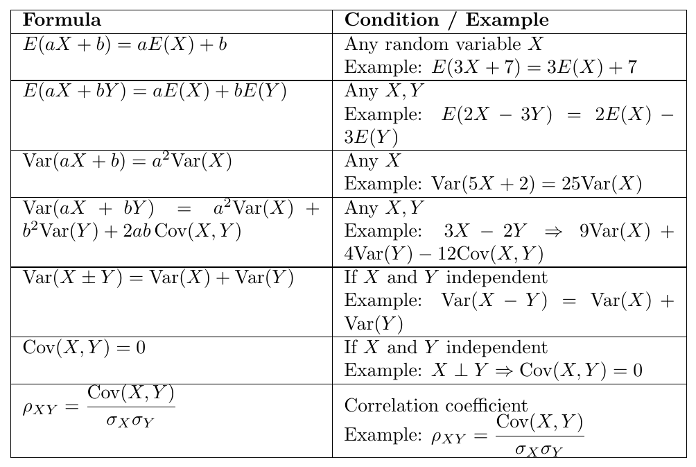
Mean and Variance of a Random Variable

Let $X$ be a random variable with probability distribution $f(x)$. The expected value or mean of $X$ is defined differently based on whether $X$ is discrete or continuous:

• Discrete case: \[ \mu = \mathbb{E}(X) = \sum_x x f(x) \]

• Continuous case: \[ \mu = \mathbb{E}(X) = \int_{-\infty}^{\infty} x f(x) \, dx \]

Let $X$ be a discrete random variable with the following probability distribution:

\[ \begin{array}{c|ccc} x & 1 & 2 & 3 \\ f(x) & 0.2 & 0.5 & 0.3 \\ \end{array} \]

Then the expected value is: \[ \mathbb{E}(X) = 1 \cdot 0.2 + 2 \cdot 0.5 + 3 \cdot 0.3 = 0.2 + 1.0 + 0.9 = 2.1 \]

Let $X$ be a continuous random variable with the probability density function: \[ f(x) = \begin{cases} 2x, & 0 < x < 1 \\ 0, & \text{otherwise} \end{cases} \]

Then the expected value is: \[ \mathbb{E}(X) = \int_0^1 x \cdot 2x \, dx = \int_0^1 2x^2 \, dx = \left[ \frac{2x^3}{3} \right]_0^1 = \frac{2}{3} \]

Problem:

A salesperson for a medical device company has two appointments on a given day.

• At the first appointment, there is a $70\%$ chance ($P_1 = 0.7$) of making a deal with a commission of $1000.

• At the second appointment, there is a $40\%$ chance ($P_2 = 0.4$) of making a deal with a commission of $1500.

• The two appointments are independent.

What is the salesperson's expected total commission based on their own probability belief?

Solution:

Let $X_1$ be the random variable representing the commission from the first appointment, and $X_2$ for the second.

\begin{align*} \mathbb{E}[X_1] &= (0.7)(1000) + (0.3)(0) = 700 \\ \mathbb{E}[X_2] &= (0.4)(1500) + (0.6)(0) = 600 \\ \text{Total Expected Commission} &= \mathbb{E}[X_1] + \mathbb{E}[X_2] = 700 + 600 = \boxed{1300} \end{align*}

So, the expected commission is $1300.

Problem:

Let $X$ be the random variable that denotes the life in hours of a certain electronic device. The probability density function is \[ f(x) = \begin{cases} \dfrac{20,000}{x^3}, & x > 100 \\ 0, & \text{elsewhere} \end{cases} \] Find the expected life of this type of device.

Solution:

The expected value (mean) of a continuous random variable $X$ with PDF $f(x)$ is: \[ \mathbb{E}[X] = \int_{-\infty}^{\infty} x f(x)\,dx \]

Since $f(x) = 0$ outside $x > 100$, we compute: \[ \mathbb{E}[X] = \int_{100}^{\infty} x \cdot \frac{20,000}{x^3} \, dx = \int_{100}^{\infty} \frac{20,000}{x^2} \, dx \]

Now compute the integral: \[ \begin{aligned} \mathbb{E}[X] &= 20,000 \int_{100}^{\infty} x^{-2} \, dx \\ &= 20,000 \left[ \frac{x^{-1}}{-1} \right]_{100}^{\infty} \\ &= 20,000 \left[ 0 - \left(-\frac{1}{100} \right) \right] \\ &= 20,000 \cdot \frac{1}{100} \\ &= \boxed{200} \end{aligned} \]

Answer: The expected life of the device is 200 hours.

Let $X$ be a random variable with probability distribution $f(x)$. The expected value of the random variable $g(X)$ is given by:

\[ \mu_{g(X)} = \mathbb{E}[g(X)] = \sum_x g(x) f(x) \quad \text{if } X \text{ is discrete} \]

and

\[ \mu_{g(X)} = \mathbb{E}[g(X)] = \int_{-\infty}^{\infty} g(x) f(x) \, dx \quad \text{if } X \text{ is continuous}. \]

Consider a random variable $X$ that denotes the number of cars arriving at a car wash in a day. The probability distribution of $X$ is:

Suppose the manager rewards the attendant according to the rule \[ g(X) = 2X - 1, \] where $g(X)$ represents the amount (in dollars) paid.

Task: Compute the expected payment to the attendant during this one-hour period.

Solution: The expected reward is \[ \mathbb{E}[g(X)] = \sum_{x=4}^{9}(2x - 1)\,P(X=x). \] \[ = (7)\left(\tfrac{1}{12}\right) + (9)\left(\tfrac{1}{12}\right) + (11)\left(\tfrac{1}{4}\right) + (13)\left(\tfrac{1}{4}\right) + (15)\left(\tfrac{1}{6}\right) + (17)\left(\tfrac{1}{6}\right). \] \[ = \tfrac{7+9}{12} + \tfrac{11+13}{4} + \tfrac{15+17}{6} = \tfrac{16}{12} + \tfrac{24}{4} + \tfrac{32}{6}. \] \[ = 1.33 + 6 + 5.33 = \boxed{\$12.67}. \]

Thus, on average, the attendant can expect to earn about $12.67 during this period.

Let $X$ be a random variable with density function \[ f(x) = \begin{cases} \frac{x^2}{3}, & -1 < x < 2 \\ 0, & \text{elsewhere} \end{cases} \]

Let $g(X) = 4X + 3$.

Find: The expected value of $g(X)$.

Solution: we have: \[ \mathbb{E}[g(X)] = \mathbb{E}(4X + 3) = \int_{-1}^{2}(4x + 3)\cdot \frac{x^2}{3} \, dx \] \[ = \frac{1}{3} \int_{-1}^{2}(4x^3 + 3x^2) \, dx = \frac{1}{3} \left[ x^4 + x^3 \right]_{-1}^{2} \]

Now compute: \[ = \frac{1}{3} \left[(2^4 + 2^3) - ((-1)^4 + (-1)^3)\right] = \frac{1}{3} \left[(16 + 8) - (1 - 1)\right] = \frac{1}{3}(24) = \boxed{8} \]

Let \( X \) and \( Y \) be random variables with joint probability distribution \( f(x, y) \).

1. Discrete Case:

If \( X \) and \( Y \) are discrete random variables, and \( g(X, Y) \) is a function of \( X \) and \( Y \), then the expected value (or mean) of \( g(X, Y) \) is given by:

\[ \mu_{g(X,Y)} = E[g(X, Y)] = \sum_x \sum_y g(x, y) \, f(x, y) \]

2. Continuous Case:

If \( X \) and \( Y \) are continuous random variables, then the expected value is given by:

\[ \mu_{g(X,Y)} = E[g(X, Y)] = \int_{-\infty}^{\infty} \int_{-\infty}^{\infty} g(x, y) \, f(x, y) \, dx \, dy \]

Notes:

• \( f(x, y) \) is the joint probability mass function (PMF) for discrete variables or joint probability density function (PDF) for continuous variables.

• \( g(x, y) \) can be any function such as \( x+y \), \( xy \), \( x^2 + y^2 \), etc.

Let $X$ and $Y$ be the random variables with joint probability distribution indicated in table. Find the expected value of $g(X,Y)=XY$.

\[ \begin{array}{c|ccc|c} x\backslash y & 0 & 1 & 2 & \text{Row Totals} \\ 0 & 3/28 & 9/28 & 3/28 & 15/28 \\ 1 & 3/14 & 3/14 & 0 & 6/14? \\ 2 & 1/28 & 0 & 0 & 1/28 \\ \text{Column Totals} & 5/14 & 15/28 & 1/28 & 1 \end{array} \] Solution:
By the definition of expected value:

\[ E(XY)=\sum_{x}\sum_{y} xy\, f(x,y) \]

Compute each term:

\[ E(XY)=(0\cdot0)f(0,0) + (0\cdot1)f(0,1) + (1\cdot0)f(1,0) + (1\cdot1)f(1,1) + (2\cdot0)f(2,0)+\cdots \]

Only the term with $x=1$ and $y=1$ contributes:

\[ E(XY) = f(1,1) = \frac{3}{14}. \]

Given: Joint probability density function: \[ f(x, y) = \begin{cases} \dfrac{x(1 + 3y^2)}{4}, & 0 < x < 2,\; 0 < y < 1 \\ 0, & \text{elsewhere} \end{cases} \]

We are asked to find the expected value: \[ E\left(\dfrac{Y}{X}\right) \]

Solution:

\[ E\left(\dfrac{Y}{X}\right) = \int_0^1 \int_0^2 \dfrac{y}{x} \cdot f(x, y) \, dx \, dy = \int_0^1 \int_0^2 \dfrac{y}{x} \cdot \dfrac{x(1 + 3y^2)}{4} \, dx \, dy \]

Simplifying the integrand: \[ = \int_0^1 \int_0^2 \dfrac{y(1 + 3y^2)}{4} \, dx \, dy \]

Since the integrand is independent of \( x \), integrate with respect to \( x \) first:

\[ = \int_0^1 \left[ \dfrac{y(1 + 3y^2)}{4} \cdot \int_0^2 dx \right] dy = \int_0^1 \dfrac{y(1 + 3y^2)}{4} \cdot 2 \, dy \]

\[ = \int_0^1 \dfrac{y(1 + 3y^2)}{2} \, dy \]

Expand and integrate:

\[ = \int_0^1 \left( \dfrac{y}{2} + \dfrac{3y^3}{2} \right) dy = \left[ \dfrac{y^2}{4} + \dfrac{3y^4}{8} \right]_0^1 = \dfrac{1}{4} + \dfrac{3}{8} = \dfrac{5}{8} \]

Final Answer: \[ E\left(\dfrac{Y}{X}\right) = \dfrac{5}{8} \]

Note: If \( g(X, Y) = X \), then the expected value \( E(X) \) can be calculated using either the joint or the marginal distribution:

Discrete Case: \[ E(X) = \sum_x \sum_y x f(x, y) = \sum_x x g(x) \] where \( g(x) \) is the marginal distribution of \( X \), obtained by summing over all values of \( y \).

Continuous Case: \[ E(X) = \int_{-\infty}^{\infty} \int_{-\infty}^{\infty} x f(x, y) \, dy \, dx = \int_{-\infty}^{\infty} x g(x) \, dx \] where \( g(x) = \int_{-\infty}^{\infty} f(x, y) \, dy \) is the marginal density of \( X \).

Similarly, for \( E(Y) \):

Discrete Case: \[ E(Y) = \sum_y \sum_x y f(x, y) = \sum_y y h(y) \] where \( h(y) \) is the marginal distribution of \( Y \).

Continuous Case: \[ E(Y) = \int_{-\infty}^{\infty} \int_{-\infty}^{\infty} y f(x, y) \, dx \, dy = \int_{-\infty}^{\infty} y h(y) \, dy \] where \( h(y) = \int_{-\infty}^{\infty} f(x, y) \, dx \) is the marginal density of \( Y \).

Let \( X \) and \( Y \) be discrete random variables with joint probability distribution given by:

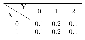
Find \( E(X) \) and \( E(Y) \).
solution:
First, compute the marginal distributions:

Marginal of \( X \): \[ P(X=0) = 0.1 + 0.2 + 0.1 = 0.4,\quad P(X=1) = 0.1 + 0.2 + 0.1 = 0.4 \]

Marginal of \( Y \): \[ P(Y=0) = 0.1 + 0.1 = 0.2,\quad P(Y=1) = 0.2 + 0.2 = 0.4,\quad P(Y=2) = 0.1 + 0.1 = 0.2 \]

Now compute expectations:

Expected value of \( X \): \[ E(X) = 0 \cdot 0.4 + 1 \cdot 0.6 = 0.6 \]

Expected value of \( Y \): \[ E(Y) = 0 \cdot 0.2 + 1 \cdot 0.4 + 2 \cdot 0.4 = 1.2 \]

Conclusion: \( E(X) = 0.6, \quad E(Y) = 1.2 \)

Let \( X \) and \( Y \) be continuous random variables with joint PDF: \[ f(x, y) = \begin{cases} 2, & 0 < x < 1,\; 0 < y < 1 \\ 0, & \text{otherwise} \end{cases} \]

Find the expected values \( E(X) \) and \( E(Y) \).

Solution:
The joint PDF is uniform over the unit square.

Marginal of \( X \): \[ g(x) = \int_0^1 f(x,y)\,dy = \int_0^1 2\,dy = 2,\quad 0 < x < 1 \]

Marginal of \( Y \): \[ h(y) = \int_0^1 f(x,y)\,dx = \int_0^1 2\,dx = 2,\quad 0 < y < 1 \]

Expected value of \( X \): \[ E(X) = \int_0^1 x \cdot 2\,dx = 2 \cdot \left[ \frac{x^2}{2} \right]_0^1 = 1 \]

Expected value of \( Y \): \[ E(Y) = \int_0^1 y \cdot 2\,dy = 2 \cdot \left[ \frac{y^2}{2} \right]_0^1 = 1 \]

Conclusion: \( E(X) = E(Y) = 1 \)

Let $X$ and $Y$ be random variables. The conditional expectation of $X$ given $Y=y$ is defined as:

\[ E[X\mid Y=y] = \sum_x x\, f(x\mid y), \quad \text{(discrete)} \]

\[ E[X\mid Y=y] = \int_{-\infty}^{\infty} x\, f(x\mid y)\, dx, \quad \text{(continuous)} \]

where the conditional probability/density is

\[ f(x\mid y) = \frac{f(x,y)}{h(y)}, \quad f(y\mid x) = \frac{f(x,y)}{g(x)} \]

and the marginals are denoted as

\[ g(x) = \sum_y f(x,y) \text{ or } \int f(x,y) dy, \quad h(y) = \sum_x f(x,y) \text{ or } \int f(x,y) dx. \]

Let $X$ take values $1,2,3$ and $Y$ indicate group membership (0 or 1). Let the joint probability be $f(x,y)$. Find $E[X\mid Y=1]$ and $E[X\mid Y=0]$. Compute the marginals:

Solution:

\[ h(y) = \sum_x f(x,y) \]

Conditional probabilities:

\[ f(x\mid y) = \frac{f(x,y)}{h(y)} \]

Then the conditional expectation:

\[ E[X\mid Y=y] = \sum_x x \, f(x\mid y) \]

Compute for $y=1$ and $y=0$ using the given table.

Given joint PMF:

\[ \begin{array}{c|cc} X\backslash Y & 0 & 1 \\ 0 & 0.2 & 0.1 \\ 1 & 0.3 & 0.4 \end{array} \]

Find $E[X\mid Y=0]$ and $E[X\mid Y=1]$ using marginals $h(y)$.

Solution:
Compute marginals:

\[ h(0) = 0.2+0.3=0.5, \quad h(1)=0.1+0.4=0.5 \]

Conditional PMFs:

\[ f(x\mid 0) = \frac{f(x,0)}{h(0)} = \{0.4,0.6\}, \quad f(x\mid 1) = \frac{f(x,1)}{h(1)} = \{0.2,0.8\} \]

Conditional expectations:

\[ E[X\mid Y=0] = 0\cdot0.4 + 1\cdot0.6 = 0.6 \]

\[ E[X\mid Y=1] = 0\cdot0.2 + 1\cdot0.8 = 0.8 \]

Let $X$ and $Y$ have joint density $f(x,y)=6x$ for $0<x<y<1$. Compute $E[X\mid Y=y]$ using marginal $h(y)$.

Solution:
Compute marginal of $Y$:

\[ h(y) = \int_0^y f(x,y)\, dx = \int_0^y 6x\, dx = 3y^2 \]

Conditional density:

\[ f(x\mid y) = \frac{f(x,y)}{h(y)} = \frac{6x}{3y^2} = \frac{2x}{y^2}, \quad 0<x<y \]

Expectation:

\[ E[X\mid Y=y] = \int_0^y x \cdot f(x\mid y)\, dx = \int_0^y x \cdot \frac{2x}{y^2} dx = \frac{2y}{3} \]

Let $f(x,y)=12 xy$ for $0<x<1,0<y<1$. Compute $E[X\mid Y=y]$ using marginal $h(y)$.

Solution:
Compute marginal of $Y$:

\[ h(y) = \int_0^1 f(x,y)\, dx = \int_0^1 12xy\, dx = 6y \]

Conditional density:

\[ f(x\mid y) = \frac{f(x,y)}{h(y)} = \frac{12xy}{6y} = 2x, \quad 0<x<1 \]

Expectation:

\[ E[X\mid Y=y] = \int_0^1 x\cdot 2x\, dx = \frac{2}{3} \]

Notice: $E[X\mid Y=y]$ is independent of $y$.

Let $X$ be a random variable with probability distribution $f(x)$ and mean $\mu$.

Variance of $X$ is given by: \[ \sigma^2 = \mathbb{E}[(X - \mu)^2] = \sum_x (x - \mu)^2 f(x), \quad \text{if $X$ is discrete,} \] \[ \sigma^2 = \mathbb{E}[(X - \mu)^2] = \int_{-\infty}^{\infty} (x - \mu)^2 f(x)\, dx, \quad \text{if $X$ is continuous.} \]

Standard Deviation of $X$ is the positive square root of the variance: \[ \sigma = \sqrt{\sigma^2} \]

The variance of a random variable \( X \) can also be computed using the formula: \[ \sigma^2 = \mathbb{E}(X^2) - \mu^2 \] where:

• \( \mathbb{E}(X^2) \) is the expected value of \( X^2 \),

• \( \mu = \mathbb{E}(X) \) is the mean of \( X \),

• \( \sigma^2 \) is the variance of \( X \).

Let \( X \) be a random variable and \( g(X) \) be a function of \( X \). Then the variance of \( g(X) \) is given by: \[ \sigma^2_{g(X)} = \mathbb{E}\left([g(X) - \mu_{g(X)}]^2\right) \] where \( \mu_{g(X)} = \mathbb{E}[g(X)] \) is the expected value of \( g(X) \).

Let $X$ be a random variable with probability distribution $f(x)$. The variance of the random variable $g(X)$ is:

\[ \sigma^2_{g(X)} = \mathbb{E}\left\{[g(X) - \mu_{g(X)}]^2\right\} = \sum_x [g(x) - \mu_{g(X)}]^2 f(x), \quad \text{if $X$ is discrete,} \]

\[ \sigma^2_{g(X)} = \mathbb{E}\left\{[g(X) - \mu_{g(X)}]^2\right\} = \int_{-\infty}^{\infty} [g(x) - \mu_{g(X)}]^2 f(x) \, dx, \quad \text{if $X$ is continuous.} \]

Let \( X \) be a random variable with the following probability distribution:

\[ \begin{array}{c|ccc} x & -2 & 3 & 5 \\ f(x) & 0.3 & 0.2 & 0.5 \end{array} \]

Step 1: Compute the mean \( \mu = \mathbb{E}[X] \) \[ \mu = (-2)(0.3) + 3(0.2) + 5(0.5) = -0.6 + 0.6 + 2.5 = 2.5 \]

Step 2: Compute \( \mathbb{E}[X^2] \) \[ \mathbb{E}[X^2] = (-2)^2(0.3) + 3^2(0.2) + 5^2(0.5) = 4(0.3) + 9(0.2) + 25(0.5) = 1.2 + 1.8 + 12.5 = 15.5 \]

Step 3: Compute variance and standard deviation \[ \sigma^2 = \mathbb{E}[X^2] - \mu^2 = 15.5 - (2.5)^2 = 15.5 - 6.25 = 9.25 \] \[ \sigma = \sqrt{9.25} \approx 3.04 \]

Let \( Y = 3X - 2 \), where \( X \) has the density function: \[ f(x) = \begin{cases} \frac{1}{4} e^{-x/4}, & x > 0 \\ 0, & \text{elsewhere} \end{cases} \]

Step 1: Mean and Variance of \( X \) (Exponential distribution)

\[ \mathbb{E}[X] = 4, \quad \text{Var}(X) = 4^2 = 16 \]

Step 2: Use linear transformation rules

\[ \mathbb{E}[Y] = \mathbb{E}[3X - 2] = 3 \cdot \mathbb{E}[X] - 2 = 3(4) - 2 = 10 \]

\[ \text{Var}(Y) = \text{Var}(3X - 2) = 3^2 \cdot \text{Var}(X) = 9 \cdot 16 = 144 \]

Given: \[ f(x) = \begin{cases} \frac{2(x+2)}{5}, & 0 < x < 1 \\ 0, & \text{otherwise} \end{cases} \quad \text{and} \quad g(X) = 3X^2 + 4 \]

Step 1: Compute \( \mu_{g(X)} = \mathbb{E}[g(X)] \)

\[ \mathbb{E}[g(X)] = \int_0^1 (3x^2 + 4) \cdot \frac{2(x+2)}{5} \, dx \]

First simplify the integrand: \[ (3x^2 + 4)(2x + 4) = 6x^3 + 8x^2 + 24x + 32 \Rightarrow \frac{1}{5} (6x^3 + 8x^2 + 24x + 32) \]

\[ \begin{aligned} \mu_{g(X)} &= \frac{1}{5} \int_0^1 (6x^3 + 8x^2 + 24x + 32) \, dx \\ &= \frac{1}{5} \left[ \frac{6x^4}{4} + \frac{8x^3}{3} + \frac{24x^2}{2} + 32x \right]_0^1 \\ &= \frac{1}{5} \left( \frac{6}{4} + \frac{8}{3} + 12 + 32 \right) \\ &= \frac{1}{5} \left(1.5 + 2.\overline{6} + 12 + 32 \right) \\ &= \frac{48.\overline{166}}{5} \\ &= \boxed{9.6334} \end{aligned} \]

Step 2: Compute \( \mathbb{E}[g(X)^2] \) (use expansion of \( g(X)^2 = (3x^2 + 4)^2 = 9x^4 + 24x^2 + 16 \))

\[ \mathbb{E}[g(X)^2] = \int_0^1 (9x^4 + 24x^2 + 16) \cdot \frac{2(x+2)}{5} \, dx \quad \text{(you can expand, integrate term-wise similarly)} \]

Then compute: \[ \sigma^2_{g(X)} = \mathbb{E}[g(X)^2] - (\mu_{g(X)})^2 \]

(This step left as exercise for integration; numerical computation follows same idea.)

Let $X$ and $Y$ be random variables with joint probability distribution $f(x, y)$. The covariance of $X$ and $Y$ is \[ \sigma_{XY} = E[(X - \mu_X)(Y - \mu_Y)] = \sum_x \sum_y (x - \mu_X)(y - \mu_Y) f(x, y) \] if $X$ and $Y$ are discrete, and \[ \sigma_{XY} = E[(X - \mu_X)(Y - \mu_Y)] = \int_{-\infty}^{\infty} \int_{-\infty}^{\infty} (x - \mu_X)(y - \mu_Y) f(x, y) \, dx \, dy \] if $X$ and $Y$ are continuous.

The covariance of two random variables $X$ and $Y$ with means $\mu_X$ and $\mu_Y$, respectively, is also given by: \[ \sigma_{XY} = E(XY) - \mu_X \mu_Y \]

Let the joint probability distribution of random variables $X$ and $Y$ be given as:

\[ \begin{array}{c|cc} X \backslash Y & 1 & 2 \\ 0 & 0.1 & 0.2 \\ 1 & 0.3 & 0.4 \\ \end{array} \]

Step 1: Find marginal probabilities

\[ P_X(0) = 0.1 + 0.2 = 0.3, \quad P_X(1) = 0.3 + 0.4 = 0.7 \] \[ P_Y(1) = 0.1 + 0.3 = 0.4, \quad P_Y(2) = 0.2 + 0.4 = 0.6 \]

Step 2: Find means

\[ \mu_X = 0 \cdot 0.3 + 1 \cdot 0.7 = 0.7 \] \[ \mu_Y = 1 \cdot 0.4 + 2 \cdot 0.6 = 1.6 \]

Step 3: Covariance formula

\[ \mathrm{Cov}(X, Y) = \sum_x \sum_y (x - \mu_X)(y - \mu_Y) f(x, y) \]

Step 4: Compute terms

\[ \begin{aligned} (0 - 0.7)(1 - 1.6)(0.1) &= (-0.7)(-0.6)(0.1) = 0.042 \\ (0 - 0.7)(2 - 1.6)(0.2) &= (-0.7)(0.4)(0.2) = -0.056 \\ (1 - 0.7)(1 - 1.6)(0.3) &= (0.3)(-0.6)(0.3) = -0.054 \\ (1 - 0.7)(2 - 1.6)(0.4) &= (0.3)(0.4)(0.4) = 0.048 \\ \end{aligned} \]

\[ \mathrm{Cov}(X, Y) = 0.042 - 0.056 - 0.054 + 0.048 = -0.02 \]

Final Answer: \( \boxed{\mathrm{Cov}(X, Y) = -0.02} \)

Let \( X \) and \( Y \) be continuous random variables with joint PDF: \[ f(x, y) = \begin{cases} 8xy, & 0 < x < 1, \, 0 < y < 1 \\ 0, & \text{otherwise} \end{cases} \]

Step 1: Compute means

\[ \mu_X = \int_0^1 x \left( \int_0^1 8xy \, dy \right) dx = \int_0^1 x \cdot 4x \, dx = 4 \int_0^1 x^2 \, dx = \frac{4}{3} \]

\[ \mu_Y = \int_0^1 y \left( \int_0^1 8xy \, dx \right) dy = \int_0^1 y \cdot 4y \, dy = 4 \int_0^1 y^2 \, dy = \frac{4}{3} \]

Step 2: Compute \( E(XY) \)

\[ E(XY) = \int_0^1 \int_0^1 xy \cdot 8xy \, dx \, dy = 8 \int_0^1 \int_0^1 x^2 y^2 \, dx \, dy = 8 \cdot \frac{1}{3} \cdot \frac{1}{3} = \frac{8}{9} \]

Step 3: Covariance

\[ \mathrm{Cov}(X, Y) = E(XY) - \mu_X \mu_Y = \frac{8}{9} - \left( \frac{4}{3} \cdot \frac{4}{3} \right) = \frac{8}{9} - \frac{16}{9} = -\frac{8}{9} \]

Final Answer: \( \boxed{\mathrm{Cov}(X, Y) = -\frac{8}{9}} \)

Let $X$ and $Y$ be random variables with covariance $\sigma_{XY}$ and standard deviations $\sigma_X$ and $\sigma_Y$, respectively. The correlation coefficient of $X$ and $Y$ is defined as \[ \rho_{XY} = \frac{\sigma_{XY}}{\sigma_X \sigma_Y}. \]

Let $X$ and $Y$ have the joint probability distribution:

\[ \begin{array}{c|ccc} X \backslash Y & 1 & 2 & 3 \\ 1 & 0.1 & 0.1 & 0.2 \\ 2 & 0.1 & 0.2 & 0.3 \\ \end{array} \]

Step 1: Compute $E(X)$ and $E(Y)$.

\[ E(X) = 1(0.1 + 0.1 + 0.2) + 2(0.1 + 0.2 + 0.3) = 1(0.4) + 2(0.6) = 1.6 \]

\[ E(Y) = 1(0.1 + 0.1) + 2(0.1 + 0.2) + 3(0.2 + 0.3) = 0.2 + 0.6 + 1.5 = 2.3 \]

Step 2: Compute $E(XY)$.

\[ E(XY) = 1\cdot1\cdot0.1 + 1\cdot2\cdot0.1 + 1\cdot3\cdot0.2 + 2\cdot1\cdot0.1 + 2\cdot2\cdot0.2 + 2\cdot3\cdot0.3 = 0.1 + 0.2 + 0.6 + 0.2 + 0.8 + 1.8 = 3.7 \]

Step 3: Covariance

\[ \text{Cov}(X, Y) = E(XY) - E(X)E(Y) = 3.7 - (1.6)(2.3) = 3.7 - 3.68 = 0.02 \]

Step 4: Compute $\sigma_X$ and $\sigma_Y$.

\[ E(X^2) = 1^2(0.4) + 2^2(0.6) = 0.4 + 2.4 = 2.8 \Rightarrow \sigma_X^2 = 2.8 - 1.6^2 = 0.24 \Rightarrow \sigma_X = \sqrt{0.24} \]

\[ \begin{aligned} E(Y^2) &= 1^2(0.2) + 2^2(0.3) + 3^2(0.5) \\ &= 0.2 + 1.2 + 4.5 = 5.9 \\ \sigma_Y^2 &= E(Y^2) - (E(Y))^2 = 5.9 - 2.3^2 = 5.9 - 5.29 = 0.61 \\ \sigma_Y &= \sqrt{0.61} \end{aligned} \]

Step 5: Correlation coefficient

\[ \rho_{XY} = \frac{\text{Cov}(X, Y)}{\sigma_X \sigma_Y} = \frac{0.02}{\sqrt{0.24}\sqrt{0.61}} \approx 0.052 \]

Let $f(x, y) = 4xy$ for $0 < x < 1$, $0 < y < 1$, and zero elsewhere. Let $X$ and $Y$ be random variables with this joint PDF.

Step 1: Compute $E(X)$, $E(Y)$:

\[ E(X) = \int_0^1 \int_0^1 x \cdot 4xy \,dy\,dx = 4 \int_0^1 x^2 \left[\int_0^1 y \,dy\right] dx = 4 \int_0^1 x^2 \cdot \frac{1}{2} dx = 2 \int_0^1 x^2 dx = 2 \cdot \frac{1}{3} = \frac{2}{3} \]

Similarly,

\[ E(Y) = \frac{2}{3} \]

Step 2: Compute $E(XY)$:

\[ E(XY) = \int_0^1 \int_0^1 xy \cdot 4xy \,dy\,dx = 4 \int_0^1 x^2 \left[\int_0^1 y^2 \,dy\right] dx = 4 \int_0^1 x^2 \cdot \frac{1}{3} dx = \frac{4}{3} \cdot \frac{1}{3} = \frac{4}{9} \]

Step 3: Covariance

\[ \text{Cov}(X, Y) = E(XY) - E(X)E(Y) = \frac{4}{9} - \left(\frac{2}{3}\right)^2 = \frac{4}{9} - \frac{4}{9} = 0 \]

Step 4: Since covariance is zero, correlation is also zero: \[ \rho_{XY} = \frac{\text{Cov}(X, Y)}{\sigma_X \sigma_Y} = 0 \]

If $a$ and $b$ are constants, then: \[ E(aX + b) = aE(X) + b \] Setting $a = 0$, we get $E(b) = b$.

Setting $b = 0$, we get $E(aX) = aE(X)$.

Let $X$ be a discrete random variable with $P(X = 1) = 0.3$, $P(X = 2) = 0.4$, $P(X = 3) = 0.3$. Find $E(2X + 3)$.

Solution: \[ E(X) = 1(0.3) + 2(0.4) + 3(0.3) = 2.0 \\ E(2X + 3) = 2E(X) + 3 = 2(2.0) + 3 = 7 \]

Let $X$ have pdf $f(x) = 2x$ for $0 < x < 1$. Find $E(5X - 4)$.

Solution: \[ E(X) = \int_0^1 x \cdot 2x \, dx = \int_0^1 2x^2 \, dx = \frac{2}{3} \\ E(5X - 4) = 5E(X) - 4 = 5\left(\frac{2}{3}\right) - 4 = \frac{10}{3} - 4 = -\frac{2}{3} \]

The expected value of the sum or difference of two functions of a random variable $X$ is the sum or difference of the expected values: \[ E[g(X) \pm h(X)] = E[g(X)] \pm E[h(X)] \]

The weekly demand for a drink is $g(X) = X^2 + X - 2$, where $X$ has the density function: \[ f(x) = \begin{cases} 2(x - 1), & 1 < x < 2 \\ 0, & \text{elsewhere} \end{cases} \]

Solution: We compute: \[ E[g(X)] = \int_1^2 (x^2 + x - 2) \cdot 2(x - 1) \, dx \] Expand the integrand: \[ (x^2 + x - 2)(2x - 2) = 2x^3 - 2x^2 + 2x^2 - 2x - 4x + 4 = 2x^3 - 6x + 4 \] Now integrate: \[ \int_1^2 (2x^3 - 6x + 4) \, dx = \left[\frac{2x^4}{4} - 3x^2 + 4x\right]_1^2 \\ = \left[\frac{2(16)}{4} - 3(4) + 8\right] - \left[\frac{2(1)}{4} - 3(1) + 4\right] \\ = (8 - 12 + 8) - (0.5 - 3 + 4) = 4 - 1.5 = 2.5 \] \[ \boxed{E[g(X)] = 2.5} \]

If $X$ and $Y$ are independent random variables, then: \[ E(XY) = E(X) \cdot E(Y) \]

Let $X$ and $Y$ be independent with: \[ E(X) = 2, \quad E(Y) = 5 \] Then: \[ E(XY) = 2 \cdot 5 = \boxed{10} \]

If $X$ and $Y$ are independent random variables, then: \[ \sigma_{XY} = \text{Cov}(X, Y) = E(XY) - E(X)E(Y) = 0 \]

Let $X$ and $Y$ be independent random variables such that: \[ E(X) = 1, \quad E(Y) = 3, \quad E(XY) = 3 \] Then: \[ \sigma_{XY} = E(XY) - E(X)E(Y) = 3 - (1)(3) = 0 \] \[ \boxed{\text{Cov}(X, Y) = 0} \]